Field Plots

Field plots are 2D Cartesian or 3D Cartesian plots. The axes in a field plot are all independent variables. In Tecplot 360, field plots can be created using any combination of the following zone layers:

By default, 2D and 3D field plots are initially displayed with Mesh and Edge zone layers:

Figure 1. A 2D mesh and edge plot.

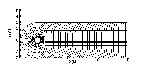
3D field plots may be enhanced with lighting effects and translucency (Translucency and Lighting).

Bounding boxes are displayed in 3D plots for volume-only zones when the plot contains only such zones and the zones themselves are not otherwise visible due to having no style. These bounding boxes may be turned off in the Options menu.

Field plots may also contain any combination of the following objects (which are derived from the values in the dataset):

This chapter discusses the plot attributes that are common to all of the plot layers.

Field Plot Modification and the Zone Style Dialog

Once you have loaded your data, you can modify field plot attributes using the Zone Style dialog or the context toolbar.

The context toolbar appears above the context menu when you right-click a zone in your field plot. This toolbar allows you to turn on or off the grid, contour, vector, shade, edge, and translucency layers for the selected zone(s). Additionally, you may adjust frequently-used style settings for each layer using the drop-down menu to the right of each, for example selecting a color for the grid (or choosing a variable by which to color it).

The Zone Style dialog may be opened by clicking the Zone Style button in the Plot sidebar or from the Plot menu. Initially, any zones selected in the workspace are selected in the Zone Style dialog. You may also double-click any zone in your plot to open the dialog with that zone selected.

Field plots containing transient data work slightly differently from static datasets in the Zone Style dialog. If a zone contains no data at the current time step, that entire line in the Zone Style dialog is grayed out. See Time Aware for more information on working with transient datasets.

The following pages are available in the Zone Style dialog, each representing a plot layer:

Mesh: See Mesh Layer.
Contour: See Contour Layer.
Vector: See Vector Layer.
Scatter: See Scatter Layer.
Shade: See Shade Layer.
Edge: See Edge Layer.
Points: See Points.
Surfaces: See Surfaces.
Volume: See Derived Volume Object Plotting. (3D only)
Effects: See Translucency and Lighting.

The values in the Zone Style dialog can be modified in place. For example, some settings, such as Show Zone, are represented by checkboxes, and can simply be clicked to toggle their state. Other settings allow you to right-click to display a context menu or other method for changing them. These allow you to change the setting for multiple zones at once by selecting the desired zones (hold down Shift or Control while clicking), then right-clicking in the column for the setting you wish to change.

Each page of the dialog is divided into three color-coded regions. The blue columns apply to the zone itself and are the same on all pages of the dialog. The green and orange columns represent primary and secondary settings specific to the corresponding plot layer.

The following attributes in the Zone Style dialog apply to the zone in general and appear on all pages of the dialog.

Zone Number: The number of each zone.
Zone Name: The name of each zone. Strands are indicated by an "*" after the name.

For transient data, the first zone of the strand applicable to the current time step is displayed in the Zone Name and Zone Number columns.

Group Number: Displays the zone’s group number. Double-click to change the number.
Show Zone: By default, all zones are displayed. Turn zones or groups of zones on or off by toggling the checkboxes in this column on or off.
Select Zones by Pattern: Enter a wildcard pattern in the Selection criteria text box and click Zones or Groups to select one or more zones based their name or group number. Selecting Zones will match the selection criteria with the Zone Name while selecting Groups will match the selection criteria with the Group Number. In wildcard patterns, most characters match themselves, but the * and ? characters have special meaning.

Character Meaning

Character	Meaning
`?`	Matches any single character.
`*`	Matches any number of characters, including none.

?

Matches any single character.

*

Matches any number of characters, including none.

Clear: Clear the selection and the Selection criteria field.

The remaining columns in the Zone Style dialog are dependent upon the active page and are discussed in their corresponding sections.

Points

You may select the source for the data points used to plot vectors and scatter symbols from the Points page of the Zone Style dialog (shown below).

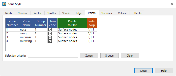
For information on using the controls at the bottom of the Zone Style dialog to select zones by name, see the description of these at the end of Field Plot Modification and the Zone Style Dialog.

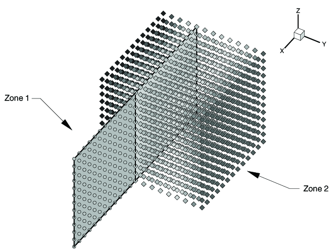
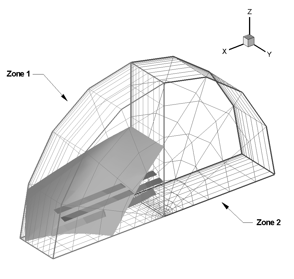
Figure 2 shows a plot where zone 1 is plotting scatter symbols only on one plane (J=5) and zone 2 is plotting all symbols.

Figure 2. A plot showing two zones set to show only J-planes equal to five, with scatter symbols plotted on the surface in zone 1 and all symbols in zone 2.

Points to Plot

Right-click to select how the points are plotted:

Nodes on Surfaces: Draws only the nodes that are on the surface of the zone.
All Nodes: Draws all nodes in the zone.
All Connected: Draws all the nodes that are connected by the node map. Nodes without any connectivity are not drawn.
Cell Centers Near Surfaces: Draws points at the cell centers which are on or near the surface of the zone.
All Cell Centers: Draws points at all cell centers in the zone.

Index Skip

Right-click to specify the skip intervals for the I, J, and K-indices. The menu options are as follows:

No Skip: Set the I, J, and K-skip intervals to one; plot all points or vectors.
Enter Skip: Specify I, J, and K-skip intervals on the Enter Index Skipping dialog.

Enter Index Skipping

Use this dialog to enter the skip intervals for the I, J, and K indices.

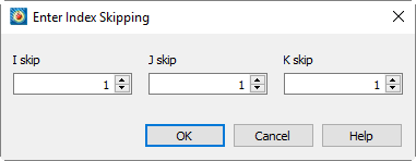
A skip value of 1 for an axis indicates that every data point along this access will be used; a skip value of 2 indicates every second data point, a skip value of 3 indicates every third data point, and so on.

For irregular and finite element data, only the I-Skip has an effect. I-skip will allow you to skip through nodes in the order they are listed in the data file.

Surfaces

There are many ways to divide volume data for plotting. One way to view volume data is to select surfaces from part of the data. In Tecplot 360 you may choose which surfaces to plot for volume zones from the Surfaces page of the Zone Style dialog (accessed by double-clicking on a zone via the Plot sidebar, or via Plot→Zone Style.

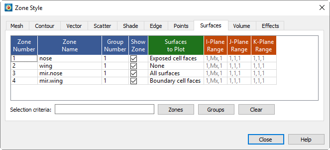
For information on using the controls at the bottom of the Zone Style dialog to select zones by name or by group number, see the description of these at the end of Field Plot Modification and the Zone Style Dialog.

Right-click in the Surfaces to Plot column to choose one of the following:

None

None of the volume zone surfaces are plotted (edges still appear). This is the default Surfaces setting for your plot.

Boundary Cell Faces

Plots all surfaces on the outside of the volume zone. This includes:

IJK-ordered data: The minimum and maximum I, J, and K-planes are plotted.
Finite element volume data: All faces that do not have a neighbor cell (according to the connectivity list) are plotted.

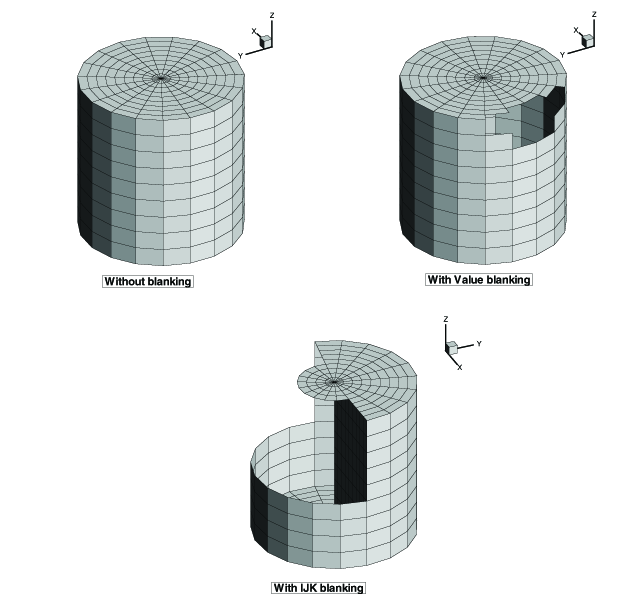
If blanking is turned on, the boundary cells in the blanked region will not be drawn and you will be able to see the interior of the volume zone. Figure 3 shows plots of a volume zone with Surfaces to Plot set to "Boundary Cell Faces": without blanking, with value blanking, and with IJK-blanking. See Blanking for information on working with Blanking.

Figure 3. Boundary Cell Face plotting without blanking, with value-blanking, and with IJK-blanking.

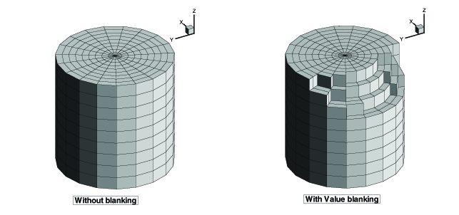
Exposed Cell Faces (default): This setting is similar to the "Boundary Cell Faces" setting, unless value blanking is active. When value blanking is used, the outer cell faces between blanked and non-blanked cells and the outer surfaces of the data are drawn. Figure 4 shows a plot of a volume zone with Surfaces to Plot set to "Exposed Cell Faces" with and without value blanking. See Blanking for information on working with Blanking.

Figure 4. Examples of plots where has been set to with (left) and without (right) value-blanking.

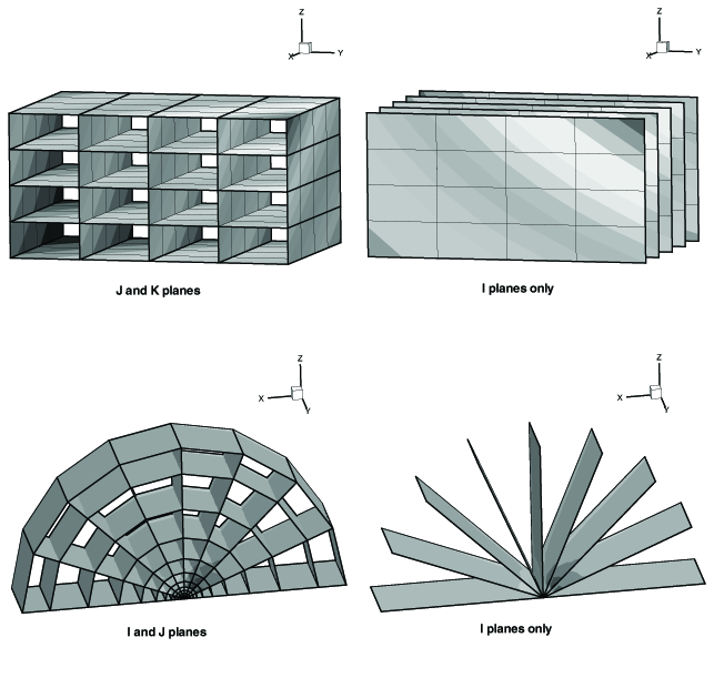
Planes Settings (I, J, K, IJ, JK, IK, and IJK-planes): Plots the appropriate combination of I, J, and/or K-planes. The planes are determined by the Range for each plane, which can be set by right-clicking in a range column. These settings are available only for IJK-ordered data. Figure 5 shows a number of examples of plotting I, J, and K-planes.

Figure 5. Examples of plotting I, J, and K-planes.

Every Surface (Exhaustive)

This setting will plot every face of every cell in volume data. It is not recommended for large datasets. Unless the surfaces are translucent, the plot will appear the same as the Exposed Cell Faces setting.

Ranges: The Range for I, J, or K Planes options allow you to specify the ranges for the corresponding planes. Right-click in the appropriate Range column to enter the range as the beginning plane, the ending plane (0 indicates the maximum index, -1 the next highest, and so on) and the skip factor in the Enter Range dialog. Use a skip factor of two to display every other plane, a skip factor of three to display every third plane, and so on.

Enter Range

The Enter Range dialog allows you to specify the I, J, or K index range in the Mapping Style or Zone Style window or when performing an integration.

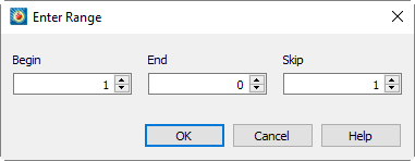
Specify the beginning and end of the range. You may specify 0 to represent the maximum index, -1 to represent the next highest, and so on.

You may also specify a skip value. A skip value of 1 considers every point in the range; 2 considers every other point, and so on.

Derived Volume Object Plotting

The Volume page of the Zone Style dialog allows you to specify whether or not to show streamtraces, iso-surfaces, or slices for the selected zone(s). Right-click in the appropriate column to choose yes or no. Figure 6 shows a plot with two zones where streamribbons and an iso-surface have been excluded from zone 2.

Figure 6. A plot where streamribbons and an iso-surface have been excluded from zone 2.

Time Aware

For transient datasets, you can use the Tecplot 360 interface to display your data at a given time or to animate your data over time. The zones loaded into Tecplot 360 can be linked to a specific solution time, and the active solution time is used to determine which zones are displayed.

For the following definitions, consider the following fictitious dataset:

Table 1. Sample Time Aware Dataset
Zone	Time	StrandID
1	n/a	n/a
2	0.0	2
3	0.18	3
4	0.22	1
5	0.25	2
6	0.28	1
7	0.32	3
8	0.38	2
9	0.42	1
10	0.52	1
11	0.57	2
12	0.58	3
13	0.62	1
14	n/a	n/a

Transient zones

Zones associated with time. The transient zone(s) displayed in the current frame are dependent upon the current solution time. Zones 2-13 in Table 1 are transient zones.

Static zones

Zones not associated with time. They are displayed regardless of the current solution time. Zones 1 and 14 from Table 1 are static.

Current Solution Time

The value that determines which transient zones are displayed in the current frame.

Strand

A series of transient zones that represent the same part of a dataset at different times. Zones 2, 5, 8, and 11 in Table 1 all have the same StrandID and therefore, they are part of the same strand.

StrandID

An integer value defined for each transient zone. The StrandID of a given zone is determined by the data loader.

Changes made in the Zone Style dialog to any zone in a given StrandID are propagated to all zones with that StrandID. See also Field Plot Modification and the Zone Style Dialog.

Relevant Zone

Only "relevant zones" are plotted at a given solution time. Tecplot provides two different policies for determining what zones are relevant at any given solution time. Please refer to $!GlobalTime TransientZoneVisibility macro command in the Scripting Guide for more information. The default option is, ZonesAtOrBeforeSolutionTime. The rules for the different transient zone visibility options are as follows:

ZonesAtOrBeforeSolutionTime: For each strand at a given solution time, the zones shown are those that are at the solution time, within a tolerance. Except for the very first or last time step, if no zones exist at the given solution time, zones shown are those from the first prior solution time showing zones.
ZonesAtSolutionTime: For each strand at a given solution time, the zones shown are those that are at the solution time, within a tolerance.

Static zones are always considered relevant. Refer to Figure 7.

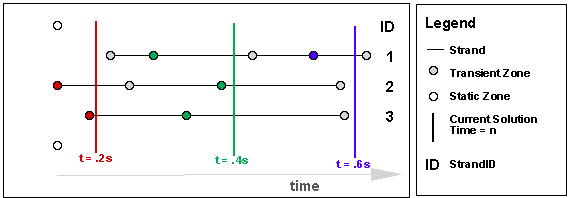
Figure 7. An illustration of how relevant zones are determined (based on the data in the figure using the default transient zone visibility, ZonesAtOrBeforeSolutionTime). For a given solution time, the relevant zones ONLY are displayed in the plot. NOTE: static zones are always considered relevant zones.

t = .2s: The red-colored transient zones and both static zones are plotted. NOTE: no zones from the first strand are represented because the strand is not defined at that time.
t = .4s: The green-colored transient zones and both static zones are plotted.
t = .6s: The blue-colored transient zones and both static zones are plotted. NOTE: no zones from the second and third strands are represented because the strands are not defined at that time.

Data Point and Cell Labels

Field Plots: You can label all or some of the data points or nodes in your field plots with either the index value(s) of the data point or the value of some specified variable at each point. You can also label each cell or element of the data with its index (which for finite element data is its element number).
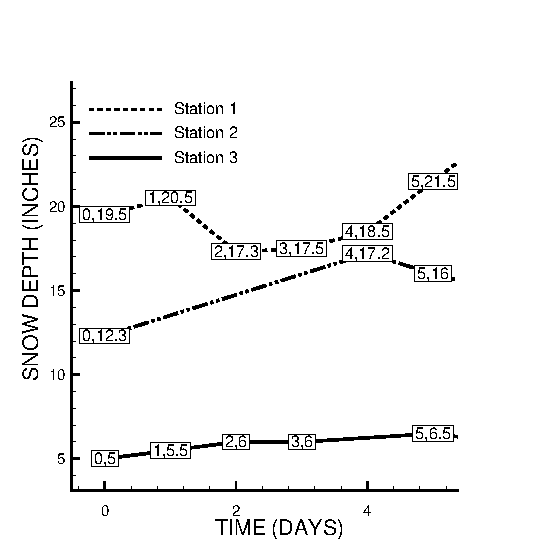
Line Plots: You can label all or some of the data points or nodes in your line plots with either the index of the data point, the value of the dependent variable at the point, or both the values (X&Y or Theta & R) for the data point. For example, Figure 8 shows an XY Line plot with each data point labeled with its X-Y value pair.

Figure 8. An XY-line plot with data labels.

To add data labels to your plot, go to Plot→Label Points and Cells dialog (accessed via the Plot menu). The Label Points and Cells dialog has the following options:

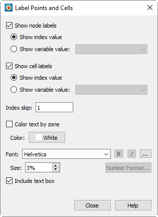
Show Node Labels

Toggle-on to show node labels. Select either Index Value or Variable Value.

Index values are not displayed for subzone data sets (.szplt) since these values cannot currently be reliably determined with this file format.

Show Cell Labels

Toggle-on to show cell labels. Select either Index Value or Variable Value.

Index Skip

If labeling by index values, select an index skip.

Color Text by Zone/Map

Toggle-on and choose the color, font, font size, and number format for the labels.

Include Text box

Toggle-on "Include Text Box" to include a box around each label.

Three-dimensional Plot Control

You can view any type of data as a 3D plot by selecting 3D Cartesian from the plot type drop-down menu in the Plot sidebar. IJK-ordered data and finite element volume data are displayed in 3D automatically.

Three-dimensional plots can be manipulated with the following controls, which can be accessed via the Plot menu:

Reset 3D Axes: Reset the 3D axis sizes and the 3D origin of rotation.
Three-dimensional Axis Limits: Control the data and axis aspect ratios for 3D plotting.
Three-dimensional Orientation Axis: Control the optional 3D orientation axis, which displays the current orientation of the three axes in the workspace.
Light Source: Control the light source position, as well as the intensity of the light, the background light, and the surface color contrast. See Three-dimensional Light Source for more details.
Advanced 3D Control: Specify the default lift fraction for 3D lines, symbols, and tangent vectors, as well as the 3D sorting algorithm for the plot.

The following controls can be accessed via the View menu.

The Rotate Dialog: Control the 3D orientation of the plot.
Three-dimensional View Details: Set the specifications for parameters affecting the 3D display of your plot, including the perspective, field of view, angular orientation of the plot, and view distance.

Reset 3D Axes

By default, the 3D axes are calculated to fit the data. If you alter your data to expand or contract the overall data size, the axes will not automatically adjust to the new size. Use the Reset 3D Axes option (accessed via the Plot menu) to reset the axes to fit the data.

The Reset 3D Axes option also resets the 3D origin. If you have modified your 3D origin using the dialog (see The Rotate Dialog for details), the option will reset it to approximately the centroid of the data.

Three-dimensional Axis Limits

In a 3D plot, whenever you read a data file, manipulate the values of variables assigned to the axes, or change variables assigned to the axes, Tecplot 360 examines the data and determines how to plot it. The data may require scaling in one or more axis directions, a change of the axis dependency, an adjustment of the space between the data and the axis box, and/or an adjustment of the shape of the axis box.

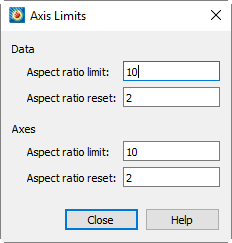
Because there are many valid forms in which the data could be plotted, by using the 3D Axis Limits dialog (accessed via the Plot menu), you can input information to help Tecplot 360 determine how to automatically configure the plot the way you want.

Aspect Ratio: Ratio of the range of the variable assigned to one axis (multiplied by the axis size factor) and the range of the variable assigned to another axis (multiplied by the axis size factor).

Data Aspect Ratio Limit: When the data aspect ratio of any two axes exceeds the Data Aspect Ratio Limit, Tecplot 360 automatically rescales the longer axis so that the new data aspect ratio is equal to the Data Aspect Ratio Reset value.

If your plots are usually unscaled (such as plots of real physical objects), you should set the data aspect ratio maximum to a large number like 30. Use a smaller number for evenly scaled axes.
Axes Aspect Ratio Limit: Works similarly to the Data Aspect Ratio Limit, except Axes Aspect Ratio Limit attends to the shape and size of the axes box.

Three-dimensional Orientation Axis

The 3D orientation axis is a representation of your axes that immediately shows you the orientation. By default, all 3D plots show the 3D orientation axis in the upper right of the frame.

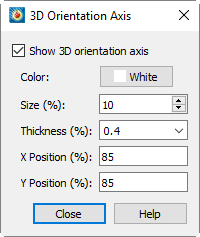
Using the 3D Orientation Axis dialog under the Plot menu, you can control whether the 3D orientation axis is shown in your plot, and if so, its color, size, line thickness, and the position of the axis origin. You can also position the 3D orientation axis by simply clicking on it and dragging the axis to the desired location in the frame.

Advanced 3D Control

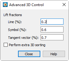
Lift Fractions: The lift fraction is the fraction of the distance from the 3D origin of the object to your eye. If you specify lift fractions for 3D lines, tangent vectors, or scatter symbols, plotted objects of the appropriate type are lifted slightly towards you so that they lie on top of surface elements.
Perform Extra 3D Sorting: For some 3D plots (i.e. plots with translucency), Tecplot 360 uses a painter’s algorithm. A quick sorting algorithm is used by default. The data objects are divided into smaller objects. The smallest object is usually a cell, finite element, vector, or scatter symbol. These objects are sorted based upon the distance from viewer, starting with the objects farthest from the viewer and working forward. This does not detect problems such as intersecting objects. If the "Perform Extra 3D Sorting" check box is selected, a slower, more accurate approach is used to detect problems for you.

There are instances when Tecplot 360 cannot sort correctly. For example, consider elements A, B, and C, where element A overlaps part of element B which overlaps part of element C which overlaps part of element A. Since Tecplot 360 draws only whole elements, one of these elements will be drawn last and each will cover (incorrectly) a portion of another element. If this occurs while printing or exporting, choosing an image format will often resolve the problem

All of the settings in the dialog are specific to the current frame.

The Rotate Dialog

You may rotate your 3D plots using the 3D Rotate dialog accessible via View→Rotate. The 3D rotation tools located in the toolbar are discussed in Three-dimensional Rotation.

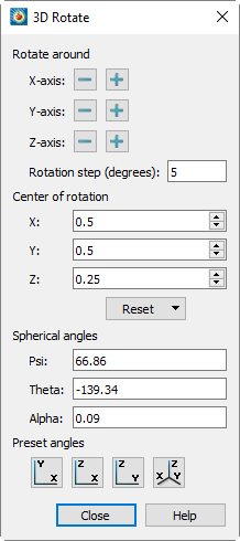
The 3D Rotate dialog has the following options:

Rotate around

Click the + or - buttons next to an axis to rotate the plot incrementally around that axis.
The Rotation Step field specifies the increment by which each click of the + or - button rotates the plot.

Center of Rotation

X

the X-axis. Enter a value in the text field, or use the increase or decrease arrows at the right to specify a value.

Y

Rotation of the eye/origin ray about the Y-axis. Enter a value in the text field, or use the increase or decrease arrows at the right to specify a value.

Z

Rotation of the eye/origin ray about the Z-axis. Enter a value in the text field, or use the increase or decrease arrows at the right to specify a value.

Reset

Use this drop-down to set the center of rotation to be the Center of Data (the center of the bounding box of the data) or Center of View (the point hit by a probe at frame coordinates 50%, 50%).

Center of View can result in an error if there is no data in the center of the frame. In this situation, the center of rotation will not move.

Spherical Angles

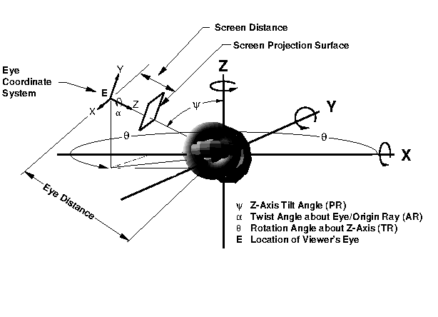
Eye origin view. The angular orientation of the plot is defined by three spherical rotation angles:

(Psi): Tilt of eye origin ray away from Z-axis. (Range –720 to 720.)
(Theta): Rotation of the eye origin ray about the Z-axis. (Range –720 to 720.)
(Alpha): Twist about the eye origin ray. (Range –720 to 720.)

The eye origin ray is a line from the origin of the 3D object to your eye. The eye origin ray is perpendicular to the plane of the computer screen. These angles define a unique view. These angles are shown in Figure 9.

Figure 9. 3D angles and 3D projection.

Preset Angles: Specify one of four pre-defined orientations: the XY-Plane, the YZ-Plane, the XZ-Plane; or a default orientation with a Psi=60, Theta=225, and Alpha=0).

Rotate About the Viewer Position

In addition to the rotation capabilities described above, you may also use the Alt key and mouse to rotate about the viewer (instead of rotating the object). Although you may use this feature while in orthographic projection, it is best suited for when perspective projection is being used. The Alt key and your middle mouse button may be used to simulate fly-through type motion. You may move closer to the object using the Alt key and middle mouse button, then turn your head using the Alt key and left mouse button.

Three-dimensional View Details

Use the 3D View Details dialog (accessed via the View menu) to control a variety of parameters affecting the display of 3D plots.

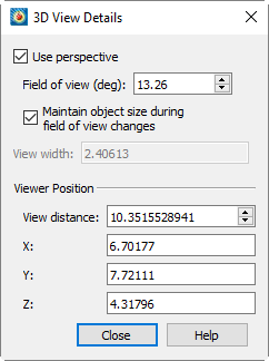
Use Perspective: Sets Tecplot 360’s projection type. If selected, Tecplot 360 draws the current frame with perspective projection. If not selected, Tecplot 360 draws the current frame with orthographic^[1] projection. (Range is 0.1 to 179.9.)
Field of View (deg): Sets the amount of the plot (in terms of spherical arc) in front of the viewer that may be seen. Zooming in or out of a 3D perspective plot changes this number and the viewer’s position.
Maintain Object Size During Field of View Changes: If selected, Field of View changes result in the viewer’s position being moved so that approximately the same amount of the plane is visible after the change.

If not selected, Field of View changes do not change the viewer’s position and result in the entire plot appearing to grow or shrink.
View Width: Sets the amount of the plot (in X-axis units) in front of the viewer that may be seen. Zooming in or out of a 3D orthographic plot changes this number, but not the viewer’s position. Not available when using perspective.
Viewer Position: Change the viewer’s relation to the image by resetting the X, Y, or Z-location, or by changing the view distance.

Three-Dimensional Zooming and Translating

Just as in all other plots, you may zoom and translate your plot using the mouse. This may be done using either the Zoom or Translate tools. For most tools, you may also use your middle and right mouse buttons (or Ctrl+right mouse button) to zoom and translate.

When the plot projection is orthographic, zooming by dragging with the middle mouse button magnifies the plot. When the plot projection is perspective, zooming by dragging with the middle mouse button changes the viewer angle, making the plot appear larger or smaller. If you want to change the viewer’s position by moving closer to or further away from an object, hold the Alt key down while using the middle mouse button or while using the 3D mouse.

Working with very large datasets may result in slow zooming, rotating, and translating. See Performance Dialog for further information on plot approximation if zoom, rotate, or translate performance is poor.

1. With orthographic projection, the shape of the objects is independent of distance. This is sometimes an "unrealistic" view, but it is often used when preserving true dimension is important (such as in drafting).