Data Structure
Tecplot 360 accommodates two different types of data: Ordered Data and Finite Element Data.
-
Ordered data is a set of points logically stored in a one, two, or three-dimensional array, where I, J, and K are the index values within the array. The number of data points is the product of all of the dimensions within the array.
-
Finite-element data is arranged in two arrays, a variable array and a connectivity matrix. The variable array is a collection of points in 2D or 3D space that are connected into polygonal or polyhedral units called elements. The connections between the nodes are defined by the connectivity matrix.
Connectivity List
A connectivity list is used to define which nodes are included in each element of an ordered or cell-based finite element zone. You should know your zone type and the number of elements in each zone in order to create your connectivity list.
The number of nodes required for each element is implied by your zone type. For example, if you have a finite element quadrilateral zone, you will have four nodes defined for each element. Likewise, you must provide eight numbers for each cell in a BRICK zone, and three numbers for each element in a TRIANGLE zone. If you have a cell that has a smaller number of nodes than that required by your zone type, simply repeat a node number. For example, if you are working with a finite element quadrilateral zone and you would like to create a triangular element, simply repeat a node in the list (e.g., 1,4,5,5).
In the example below, the zone contains two quadrilateral elements. Therefore, the connectivity list must have eight values. The first four values define the nodes that form Element 1. Similarly, the second four values define the nodes that form Element 2.
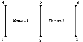
The connectivity list for this example would appear as follows:
ConnList[8] = {4,5,2,1,  /* nodes for Element 1 */
5,6,3,2}; /* nodes for Element 2 */| It is important to provide your node list in either a clockwise or counter-clockwise order. Otherwise, your cell will twist, and the element produced will be misshapen. |
Ordered Data
Ordered data is defined by one, two, or three-dimensional logical arrays, dimensioned by IMAX, JMAX, and KMAX. These arrays define the interconnections between nodes and cells. The variables can be either nodal or cell-centered. Nodal variables are stored at the nodes; cell-centered values are stored within the cells.
- One-dimensional Ordered Data (I-ordered, J-ordered, or K-ordered)
-
A single dimensional array where either IMAX, JMAX or KMAX is greater than or equal to one, and the others are equal to one. For nodal data, the number of stored values is equal to
IMAX * JMAX * KMAX. For cell-centered I-ordered data (where IMAX is greater than one, and JMAX and KMAX are equal to one), the number of stored values is (IMAX-1) - similarly for J-ordered and K-ordered data. - Two-dimensional Ordered Data (IJ-ordered, JK-ordered, IK-ordered)
-
A two-dimensional array where two of the three dimensions (IMAX, JMAX, KMAX) are greater than one, and the other dimension is equal to one. For nodal data, the number of stored values is equal to
IMAX * JMAX * KMAX. For cell-centered IJ-ordered data (where IMAX and JMAX are greater than one, and KMAX is equal to one), the number of stored values is(IMAX-1)(JMAX-1)- similarly for JK-ordered and IK-ordered data. - Three-dimensional Ordered Data (IJK-ordered)
-
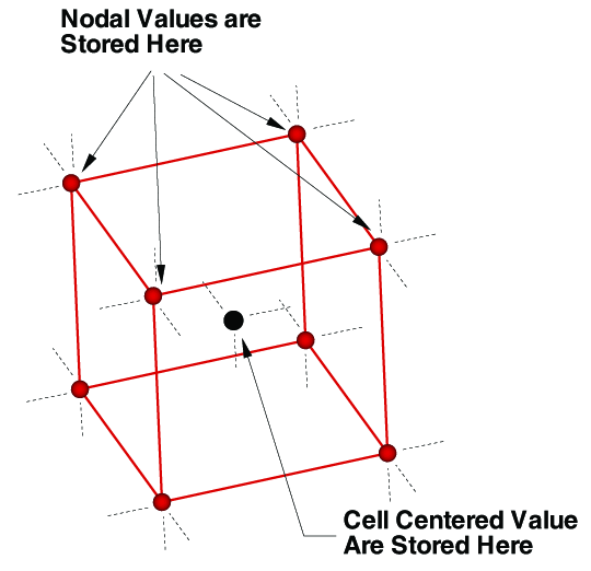 A three-dimensional array where
all IMAX, JMAX and KMAX are each greater than one. For nodal ordered data, the
number of nodes is the product of the I-, J-, and K-dimensions. For nodal data, the
number of stored values is equal to
 IMAX * JMAX * KMAX. For cell-centered data, the number of stored values is(IMAX-1)(JMAX-1)(KMAX-1).
Indexing Nodal Ordered Data
For nodal ordered data, the n-dimensional array of values are treated as a one
dimensional array. For example, given an IJK-ordered zone dimensioned by 10x20x30. To
access the value at I=3, J=4, K=5 (one based) you would use:
IMax       = 10
JMax       = 20
KMax       = 30
I       = 3
J       = 4
K       = 5
NodeIndex = I + (J-1)*IMax + (K-1)*IMax*JMax
Indexing Cell-centered Ordered Data
For cell-centered ordered data, the index that represents the cell center is the same as the nodal index that represents the lowest indexed corner of the cell.
For example, the figure below shows an IJ-ordered zone dimensioned 3x4.
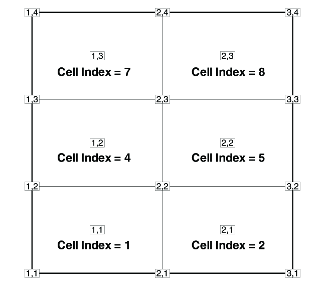
To access a cell-centered value for the cell in the upper right hand corner, use the following:
IMax      = 3
JMax      = 4
KMax      = 1
I      = 2
J      = 3
K      = 1
CellIndex    = I + (J-1)*IMax + (K-1)*IMax*JMax
You’ll notice that the equations are exactly the same as with nodal data. As a result there are gaps of unused values at IMax, JMax, and KMax that must be left unassigned.
The above equation is generic for 1D, 2D and 3D data. It simplifies for the lower dimensions.
One-dimensional Ordered Data (I, J, or K)
Values for XY Line plots are usually arranged in a one-dimensional array indexed by one parameter: I for I-ordered, J for J-ordered, or K for K-ordered, with the two remaining index values equal to one.
At each node, N variables (V1, V2, …, VN) are defined. If you arrange
the data in a table where the values of the variables (N values) at a node are given
in a row, and there is one row for each node, the table would appear something like
that shown below.
| V1 | V2 | V3 | … | VN | (Values at node I = 1) |
|---|---|---|---|---|---|
V1 |
V2 |
V3 |
… |
VN |
(Values at node I = 2) |
V1 |
V2 |
V3 |
… |
VN |
(Values at node I = 3) |
V1 |
V2 |
V3 |
… |
VN |
|
V1 |
V2 |
V3 |
… |
VN |
|
V1 |
V2 |
V3 |
… |
VN |
(Values at node I = IMax) |
See XY and Polar Line Plots for more information on XY plots.
IJK-ordered Data Plotting
In one or two-dimensional datasets, all data points are typically plotted. However, for IJK-ordered data you can designate which surface will be plotted by using the Surfaces page of the dialog. You may choose to plot just outer surfaces, or you may select combinations of I, J, and K-planes to be plotted. Refer to Surfaces for in-depth information.
Logical versus Physical Representation of Data
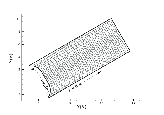
A family of I-lines results by connecting all of the points with the same I-index, similarly for J-lines and K-lines. For IJ-ordered data, both families of lines are plotted in a two-dimensional coordinate system resulting in a 2D mesh. When both the I and J-lines are plotted in a three-dimensional coordinate system, a 3D surface mesh plot results. An example of both meshes is shown below. As you can see, logical data points can transform into an arbitrary shape in physical space.
Finite Element Data
While finite element data is usually associated with numerical analysis for modeling complex problems in 3D structures (heat transfer, fluid dynamics, and electromagnetics), it also provides an effective approach for organizing data points in or around complex geometrical shapes. For example, you may not have the same number of data points on different lines, there may be holes in the middle of the dataset, or the data points may be irregularly (randomly) positioned. For such difficult cases, you may be able to organize your data as a patchwork of elements. Each element can be independent of the other elements, so you can group your elements to fit complex boundaries and leave voids within sets of elements. The figure below shows how finite element data can be used to model a complex boundary.
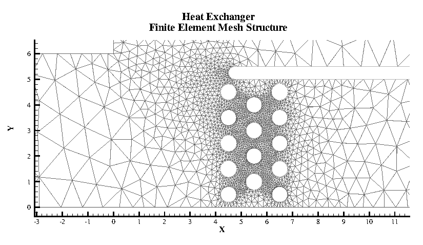
Finite element data defines a set of points (nodes) and the connected elements of these points. The variables may be defined either at the nodes or at the cell (element) center. Finite element data can be divided into three types:
-
Line data is a set of line segments defining a 2D or 3D line. Unlike I-ordered data, a single finite element line zone may consist of multiple disconnected sections. The values of the variables at each data point (node) are entered in the data file similarly to I-ordered data, where the nodes are numbered with the I-index. This data is followed by another set of data defining connections between nodes. This second section is often referred to as the connectivity list. All elements are lines consisting of two nodes, specified in the connectivity list.
-
Surface data is a set of triangular, quadrilateral, or polygonal elements defining a 2D field or a 3D surface. When using polygonal elements, the number of sides may vary from element to element. In finite element surface data, you can choose per zone to arrange your data in three-point (triangle), four-point (quadrilateral), or variable-point (polygonal) elements. The number of points per node and their arrangement are determined by the element type of the zone. If a mixture of quadrilaterals and triangles is necessary, you may repeat a node in the quadrilateral element type to create a triangle, or you may use polygonal elements.
-
Volume data is a set of tetrahedral, brick, or polyhedral elements defining a 3D volume field. When using polyhedral elements, the number of sides may vary from element to element. Finite element volume cells may contain four points (tetrahedron), eight points (brick), or a variable number of points (polyhedral). The figure below shows the arrangement of the nodes for tetrahedral and brick elements. The connectivity arrangement for polyhedral data is governed by the method in which the polyhedral facemap data is supplied.
Table 2. Connectivity arrangements for FE-volume datasets 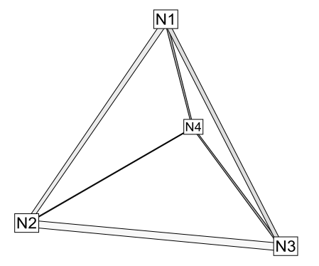
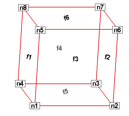
Tetrahedral connectivity arrangement
Brick connectivity arrangement
In cell-based element types (triangular, quadrilateral, tetrahedal, or brick), points
may be repeated to achieve elements containing a smaller number of points. For example,
a connectivity list of n1 n1 n1 n1 n5 n6 n7 n8 (where n1 is repeated four times)
results in a brick-based pyramid element. Any of the points could be repeated; for
example, n1 n1 n3 n3 n5 n5 n7 n7 would also be a valid way to define a pyramidal
element in a brick zone.
In Tecplot 360, each FE data zone must be composed exclusively of one element type. However, you may use a different data point structure for each zone within a dataset, as long as the number of variables defined at each data point is the same.
The Data Format Guide provides detailed information about how to format your FE data in Tecplot’s text file format.
Finite Element Data Limitations
Working with finite element data has some limitations:
-
XY-plots of finite element data treat the data as I-ordered; that is, the connectivity list is ignored. Only nodes are plotted, not elements, and the nodes are plotted in the order in which they appear in the data file.
-
Index skipping in vector and scatter plots treats finite element data as I-ordered; the connectivity list is ignored. Nodes are skipped according to their order in the data file.
Variable Location (Cell-centered or Nodal)
Data values can be stored at the nodes or at the cell centers.
-
For finite element meshes, cell-centers are the centers (centroids) of elements.
-
For many types of plots, cell-centered values are interpolated to the nodes internally.
Face Neighbors
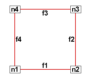
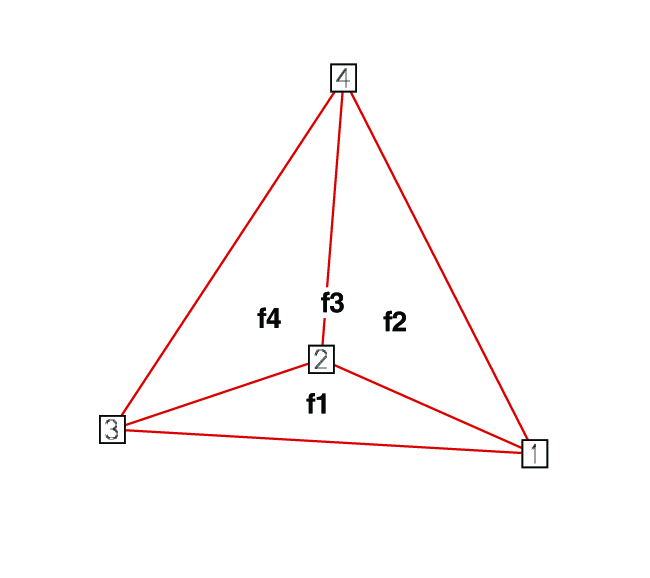
A cell is considered a neighbor if one of its faces shares all nodes in common with the selected cell, or if it is identified as a neighbor by face neighbor data in the dataset. The face numbers for cells in the various zone types are defined below.
Examples of face neighbors for various zone types.
|
A: Example of node and face neighbors for an FE-brick cell or IJK-ordered cell. |
|
B: Example of node and face numbering for an IJ-ordered/FE-quadrilateral cell. |
|
C: Example of tetrahedron face neighbors. |
The implicit connections between elements in a zone may be overridden, or connections between cells in adjacent zones established, by specifying face neighbor criteria in the data file. Refer to TECFACE in the Data Format Guide for additional information.
Working with Unorganized Datasets
Tecplot 360 loads unorganized data as a single I-ordered zone and displays them in XY Mode, by default. An I-ordered zone is considered irregular if it has more than one dependent variable. An I-ordered data set with one dependent variable (i.e. an XY or polar line) is not an irregular zone.
To check for irregular data, you can go to the dialog (accessed via the menu). The values assigned to: IMax, JMax, and KMax are displayed in the lower left quadrant of that dialog. If IMax is greater than 1, and JMax and KMax are equal to 1, then your data is irregular.
It is also easy to tell if you have irregular data by looking at the plot. If you are looking at irregular data with the Mesh layer turned on, the data points will be connected by lines in the order the points appear in the data set.
You can organize your data set for Tecplot 360 in the following ways.
-
Manually order the data file using a text editor.
Use the feature from the menu to see if your data set can be easily corrected using a text editor by correcting the values for I, J, and/or K. -
Use one of the options. See Data Interpolation.
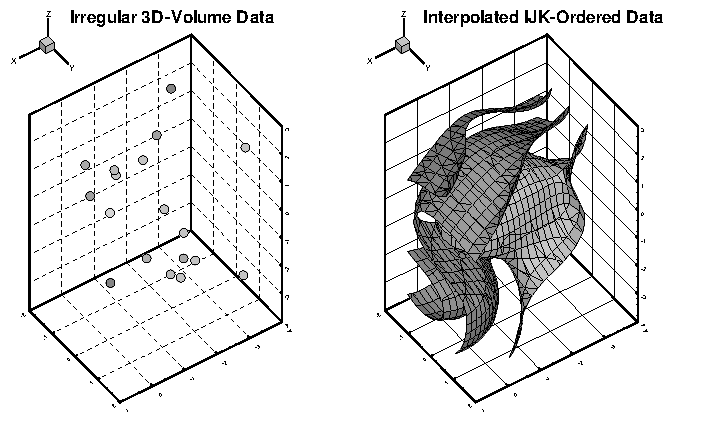
Example: Unorganized Three-Dimensional Volume
To use 3D volume irregular data in field plots, you must interpolate the data onto a regular, IJK-ordered zone. To interpolate your data, perform the following steps:
-
Place your 3D volume irregular data into an I-ordered zone in a data file.
-
Read in your data file and create a 3D scatter plot.
-
From the menu, choose . ( will also work.)
-
In the dialog, enter the I-, J-, and K-dimensions for the new zone; at a minimum, you should enter 10 for each dimension. The higher the dimensions, the finer the interpolation grid, but the longer the interpolating and plotting time.
-
Enter the minimum and maximum X, Y, and Z values for the new zone. The default values are the minimums and maximums of the current (irregular) dataset.
-
Click to create the new zone, and to dismiss the dialog.
-
From the menu, choose . Kriging may also be used.
-
In the interpolation dialog, choose the irregular data zone as the source zone, and the newly created IJK-ordered zone as the destination zone. Set any other parameters as desired (see Data Interpolation for details).
-
Select the button to perform the interpolation.
Once the interpolation is complete, you can plot the new IJK-ordered zone as any other 3D volume zone. You may plot iso-surfaces, volume streamtraces, and so forth. At this point, you may want to deactivate or delete the original irregular zone so as not to conflict with plots of the new zone.
Figure 4 shows an example of irregular data interpolated into an IJK-ordered zone, with iso-surfaces plotted on the resultant zone.
