Data Operations
Plots in Tecplot 360 rely on the datasets attached to each frame. You can modify, create, transform, interpolate, duplicate, and delete the data in the current dataset using the menu. You can also use the data operation capabilities of Tecplot 360 to create plots of analytical functions. By using layout files, macros, and/or equation files, you can create complex data operations that can be repeated on different datasets.
Changes to the dataset within Tecplot 360 do not affect the original data file(s). You can save the modified data by choosing Write Data from the menu. When you save a layout file, a journal of data operations is saved and those operations are repeated when the layout file is read at a later time. If the data in the file has changed, or the data file is overwritten with new data, the operations are applied to the new data. Alternatively, any datasets that have been modified are also saved to data files (see Layout Files and Layout Package Files for details).
Data Alteration through Equations
Use (or click the
 toolbar button) to alter
data in existing zones. The dialog allows you to change
the values of entire variables or specific data points. You can also use
this dialog to create new variables.
Changes made to the dataset in the dialog are not made to the original data file. You can save the changes by saving a layout file or writing the new data to a file. Saving a layout file will keep your data file in its original state, but use journaled commands to reapply the equations.
Variables defined in your data
file, or variables you create yourself, are referenced in equations by
surrounding them with curly braces, like {RPM}. This syntax must be
used even when first defining a variable, for example {RPM} = {RPS} * 60
to define a new RPM variable from an existing RPS variable. Variable
and function names provided by Tecplot 360 do not require the braces.
|
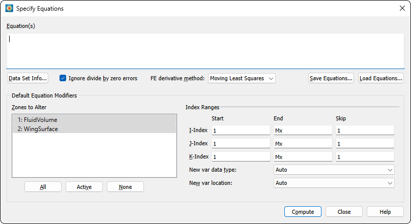
The dialog has the following options and fields:
- Equation(s)
-
Enter the equation(s) using the syntax described in Equation Syntax.
- Data Set Info
-
Opens the Data Set Info dialog (see Data Set Information).
- Ignore divide by zero errors
-
When activated, suppresses the error dialog and returns the largest or smallest possible value depending on the sign of the dividend when a divide by zero condition occurs. 0/0 will return 0.
- FE derivative method
-
Select the preferred method to use for computing finite-element derivatives. The default is Moving Least Squares. If Green-Gauss is selected, an information icon will appear to the right of the selector. Hovering the mouse over this icon will display the following information about when the calculation will fall back to the Moving Least Squares method.
The Green-Gauss method will be preferred for calculating derivatives of finite elements. The calculation will fall back to Moving Least Squares for polygonal or polyhedral elements or higher order elements. Moving Least Squares will also be used for second or higher order derivatives or when the frame dimensionality does not match the element dimensionality. For example, in 3D frame mode derivatives of surface zones will use moving least squares. - Save Equations
-
Save all equations in the Equation(s) field to a text file with an .eqn format.
- Load Equations
-
Load an equation file previously saved.
- Zones to Alter
-
Select which zones to alter. You can manually select the zones in the list (holding Shift when clicking to create a range, or Control to toggle individual zones on or off). You may use the buttons below the list to select all zones, all active zones, or no zones.
When creating a new variable, if all zones are not selected, Tecplot will create a passive variable as a placeholder for any zones that are not included in the data alteration since all zones in a dataset must have the same number of variables. Passive variables effectively return zero for every point or cell value, do not consume any memory, and can be replaced at any time with other data alterations. - Index Ranges
-
Select the index ranges to alter in the selected zones. You may skip this step if you want to apply the equation to all points of the selected zones. Use the special value
0orMxto specify the maximum index. You can also use the valuesMx-1(to specify the index one less than the maximum index),Mx-2, and so forth.For Ordered Data, the I-Index, J-Index, and K-index options correspond to the I, J, and K values in the dataset. For finite element data, the I-Index corresponds to the range of nodes and the J-Index corresponds to the cell-centered values. The K-index has no bearing on finite element data.
The Skip field indicates the increment between indices. 1 means apply the calculation to every data point, 2 means to every other data point, 3 to every third point, and so on. When creating a new variable, the new variable’s value is set to zero at any index value that is skipped.
- New Var Data Type
-
(if applicable) - Select the data type of the new variable. The following data types are available:
- Auto
-
Tecplot 360 assigns the data type based upon the variables used in the right-hand side of the equation.
- Single
-
Four-byte floating point values.
- Double
-
Eight-byte floating point values.
- Long Int
-
Four-byte integer values.
- Short Int
-
Two-byte integer values.
- Byte
-
One-byte unsigned integer values (can contain values from zero to 255).
- Bit
-
Either zero or one.
- New Var Location
-
(if applicable) - Select the location of the new variable. The options are:
- Auto
-
(default) - "Auto" is set to node unless all variables in the equation are located at the cell center.
- Node
-
Stores variable with nodal information. (see Indexing Nodal Ordered Data).
- Cell-Center
-
Stores variable with nodal information. (see Indexing Cell-centered Ordered Data).
- Compute
-
Click the Compute button to alter the data. If an error occurs during the alteration (because of division by zero, overflow, underflow, etc.), an error message is displayed, all of the zones are restored to their previous state as of the beginning of processing that equation, and processing stops. The results of equations that have been successfully processed, however, are retained.
For example, if you enter three equations, and the second contains an error, the final state is the result of processing only the first equation. The second equation is rolled back due to the error, and the third is not processed at all.
Every time you hit the [Compute] button, the equations are calculated. Be sure to remove previously computed equations before computing new ones.
Equation Syntax
You can enter multiple equations in the Equation(s) text field of the dialog. Each equation occupies one line of the text field as demarcated by the Enter key (not necessarily by where they wrap in the text field). The equations are applied in order to all specified zones and data points.
Tecplot 360 equations have the following form:
LValue = F(RValue1, RValue2, RValue3,…)
Where:
F() - A mathematical expression. |
LValue - An existing or new variable. |
RValueN - A value (such as a constant, variable value, or index value). |
If LValue already exists in the dataset of the active frame, the equation is used to modify that variable. (The same variable may be used on the right side of the equation to refer to the pre-calculation value and thereby modify it based on its original value.) If the variable does not already exist, the equation is used to create a new variable as a function of existing variables.
There may be any number of spaces within the equation. However, there cannot be any spaces between the letters of intrinsic-function names nor in variables referred to by name. (See Equation Operators and Functions.)
Equation Variables and Values
A variable is specified in one of the following ways:
- Its order in the data file
-
A variable may be referenced according to its order in the data file, where
V1is the first variable in the data file,V2is the second, and so forth.To create a new variable using this specification, you must specify the number of the next available variable (i.e. if there are 5 variables in the dataset), the new variable must be called
V6. You will receive an error message, if you attempt to assign an invalid variable number.You can confirm the number and order of variables in the data file in the dialog (choose ). The variables in the dataset are listed on the right-hand side of the page. - By its name
-
To reference a variable by its name, enclose the name with curly braces (
{and}). For example, to setV3equal to the value of the variable named R/RFR, you can enter:V3 = {R/RFR}Variable names are not case sensitive. Leading and trailing spaces are also not considered. However, spaces within the variable name are significant.
If two or more variables have the same name, the first variable is used when the variable is referred to by name. So, if both
V5andV9are namedR/rfr,V5is used.The curly braces can also be used on the left-hand side of the equation. In this case, if a variable with that name does not exist, a new variable is created with that name for all zones.
- By a letter code
-
Variables and index values may be referenced by the following letter codes:
I
Depends on the data type and the new variable’s ‘New Var Location’ value:
-
Ordered data:
-
If ‘New Var Location’ is set to ‘Node’, I is the I index number of a node.
-
If ‘New Var Location’ is set to ‘Cell center’, I is the lowest I index associated with the cell.
-
-
FE data:
-
If ‘New Var Location’ is set to ‘Node’, I is the node index number.
-
If ‘New Var Location’ is set to ‘Cell center’, I is 1.
-
J
Depends on the data type and the new variable’s ‘New Var Location’ value:
-
Ordered data:
-
If ‘New Var Location’ is set to ‘Node’, J is the J index number of a node.
-
If ‘New Var Location’ is set to ‘Cell center’, J is the lowest J index associated with the cell.
-
-
FE data:
-
If ‘New Var Location’ is set to ‘Node’, J is 1.
-
If ‘New Var Location’ is set to ‘Cell center’, J is the element number.
-
K
Depends on the data type and the new variable’s ‘New Var Location’ value:
-
Ordered data:
-
If ‘New Var Location’ is set to ‘Node’, K is the K index number of a node.
-
If ‘New Var Location’ is set to ‘Cell center’, K is the lowest K index associated with the cell.
-
-
FE data:
-
If ‘New Var Location’ is set to ‘Node’, K is 1.
-
If ‘New Var Location’ is set to ‘Cell center’, K is 1.
-
X
The variable assigned to the X-axis. In XY-plots, all active mappings must have the same X-variable in order for this variable name to be valid.
Y
The variable assigned to the Y-axis. In XY-plots, all active mappings must have the same Y-variable in order for this variable name to be valid.
Z
The variable assigned to the Z-axis (if in 3D Cartesian).
A
The variable assigned to the Theta-axis for Polar plots. For this variable to be valid, the plot type must be set to Polar Line. In addition, all active mappings must have the same Theta-variable.
R
The variable assigned to the R-axis for Polar plots. The plot type must be Polar Line, and all active mappings must have the same R-variable for this variable name to be valid.
U
The X-component of vectors (if defined).
V
The Y-component of vectors (if defined).
W
The Z-component of vectors (if defined).
B
The value-blanking variable for the first active constraint (if applicable).
C
The contour variable for contour group 1 (if defined in the dialog).
S
The scatter-sizing variable (if defined in the dialog).
SOLUTIONTIME
The current solution time.
ZONENUM
The current zone number.
MINX, MAXX
The minimum or maximum value of the variable assigned to the x-axis of the plot, for all active zones.
MINY, MAXY
The minimum or maximum value of the variable assigned to the y-axis of the plot, for all active zones.
MINZ, MAXZ
The minimum or maximum value of the variable assigned to the z-axis of the plot, for all active zones (if plot type is 3D Cartesian.)
MINU, MAXU
The minimum or maximum of the variable assigned to vector variable U, from all active zones (if vector variable U has been set.)
MINV, MAXV
The minimum or maximum of the variable assigned to vector variable V, from all active zones (if vector variable V has been set.)
MINW, MAXW
The minimum or maximum of the variable assigned to vector variable W, from all active zones (if vector variable W has been set.)
MINC, MAXC
The minimum or maximum of the variable assigned to contour group 1 for all active zones (if defined in the dialog).
MINS, MAXS
The minimum or maximum of the variable assigned to scatter-sizing variable, from all active zones (if defined in the dialog).
MAXI
If data is Ordered, returns the maximum index of dimension I for each active zone. If data is Finite Element, returns the number of points for each active zone.
MAXJ
If data is Ordered, returns the maximum index of dimension J for each active zone. If data is Finite Element MAXJ = 1.
MAXK
If data is Ordered, returns the maximum index of dimension K for each active zone. If data is Finite Element MAXK = 1.
Letter codes may be used anywhere on the right-hand side of the equation. Do not enclose them in curly braces.
Those letter codes representing variables (all letter codes except
I,J, andK) may be used on the left-hand side of the equation as well.The variables referenced by the letter codes are for the current frame.
-
Equation Operators and Functions
Binary Operators
In an equation, the valid binary operators are as follows:
+ |
Addition |
- |
Subtraction |
* |
Multiplication |
/ |
Division |
** |
Exponentiation |
Binary operators have the following precedence:
** |
Highest precedence |
*,/ |
|
+,- |
Lowest precedence |
Operators are evaluated from left to right within a precedence level.
Functions
The following functions are available. Arguments may be variables, constants, expressions, other functions.
SIN(X) |
Sine of X (must be specified in radians) |
COS(X) |
Cosine of X (must be specified in radians) |
TAN(X) |
Tangent of X (must be specified in radians) |
ABS(X) |
Absolute value of X |
ASIN(X) |
Arcsine of X (result given in radians) |
ACOS(X) |
Arccosine of X (result given in radians) |
ATAN(X) |
Arctangent of X (result given in radians) |
ATAN2(A,B) |
Arctangent of A/B (result given in radians) |
SQRT(X) |
Returns the positive square root of X |
LOG(X), ALOG(X) |
Natural logarithm (base e) of X. Both forms are equivalent. |
LOG10(X), ALOG10(X) |
Logarithm base 10 of X. Both forms are equivalent. |
EXP(X) |
Exponentiation (base e); EXP(X)= |
MIN(A, B) |
Minimum of A or B |
MAX(A, B) |
Maximum of A or B |
SIGN(X) |
Returns -1 if X is negative, +1 otherwise |
ROUND(X) |
Round X to the nearest integer |
TRUNC(X) |
Remove fractional part of X |
RAND(N) |
Returns random number between 1 and N inclusive, different for each element in the variable |
Conditional Expressions
Conditional expressions may be written using the IF function.
IF(P,T,F)If the predicate expression P is true (has a non-zero value), returns the value of expression T, otherwise returns the value of expression F. Both T and F are fully evaluated regardless of the value of P; there is no "short-circuiting."
The predicate expression may include comparison and Boolean operators, as summarized in the following table.
| Operator | Description | Example |
|---|---|---|
== |
Equal To |
{A} = IF(X==2.0, 3, 4) assigns to variable A: 3 if X equals 2.0, otherwise 4 |
!= |
Not Equal To |
{A} = IF(X != Y,Z,2) assigns to variable A: Z if X does not equal Y, otherwise 2 |
> |
Greater Than |
{A} = IF(X > 1.0, 4, 5) assigns to variable A: 4 if X > 1.0, otherwise 5 |
>= |
Greater Than or Equal To |
{A} = IF(X >= Y, 4, Z) assigns to variable A: 4 if X >= Y, otherwise Z |
< |
Less Than |
{A} = IF(X < Y, 4, Z) assigns to variable A: 4 if X < Y otherwise Z |
<= |
Less Than or Equal To |
{A} = IF(X <= Y, 4, Z) assigns to variable A: 4 if X <= Y, otherwise Z |
&& |
Logical AND |
{A} = IF(X < Y && X > 3, 8,9) assigns to variable A: 8 if X < Y AND X > 3, otherwise 9 |
|| |
Logical OR |
{A} = IF(X == 2 || X > 3, 5,6) assigns to variable A: 5 if X == 2 OR X > 3, otherwise 6 |
These operators are valid only within the first argument of an
IF function. They may not be used elsewhere in an
expression. For example, {A} = X > 1 is invalid. Instead, use {A} = IF(X > 1, 1, 0) or similar.
Python-style operator chaining (such as A < B < C) is not
supported. Although this construction is syntactically valid, it will
not produce the expected result. Use A < B && B < C instead.
&& has a higher precedence than (will be evaluated before) ||. When in doubt, use parentheses.
Derivative and Difference Functions
The derivative functions can be called in the same manner as intrinsic functions. Derivative and difference functions can be calculated with respect to the following variables:
| Variable | Definition | Restricted to: |
|---|---|---|
x, y, z |
variable assigned to the x-axis, y-axis or z-axis, respectively |
XY Line[1], or 3D |
a |
variable assigned to the theta-axis |
Polar Line |
r |
variable assigned to the radial-axis |
Polar Line |
i, j, k |
index range |
Ordered Zones |
The complete set of first and second-derivative and difference functions are listed below:
| Type | Function Calls | Applicable Variables |
|---|---|---|
First Order |
ddx, ddy, ddz, dda, ddr |
x, y, z, a, or r |
Second Order |
d2dx2, d2dy2, d2dz2, d2da2, d2dr2 |
x, y, z, a or r |
Second-Order (cross derivatives) |
d2dxy, d2dyz, d2dxz, d2dar |
xy, yz, xz, or ar |
The derivative function
ddx is used to calculate ;
d2dx2 calculates .
Type |
Function Calls |
Applicable Variables |
First Order |
ddi, ddj, ddk |
i, j, or k |
Second Order |
d2di2 d2dj2, d2dk2 |
i, j, or k |
Second Order (cross derivatives) |
d2dij, d2djk, d2dik |
ij, jk, or ik |
The difference functions ddi, d2di2, and so
forth, calculate centered differences of their argument with respect to
the indices I, J, and K based on the indices of the point. For
example:
For ordered zones, spatial derivative functions are calculated using the chain rule with difference functions. For example:
or:
The spatial derivatives of indices, such as ddx(i), are calculated from their inverses, such as ddi(x), using standard curvilinear coordinate transformations.
For finite-element zones, spatial derivatives can be calculated using either the Moving Least-Squares technique or the Green-Gauss method. For Moving Least-Squares, the variable at a particular node or cell center is assumed to vary quadratically in space about that point, and least-squares is used with all nodes surrounding the point to fit a polynomial function, whose coefficients then become the first and second derivatives of the variable. The Green-Gauss method uses surface intergals to compute derivatives and can give a better estimate of derivates for highly stretched and/or skewed grids. Note that there are limitations on when Green-Gauss will be used (see FE derivative method).
Boundary Values
Boundary values for first-derivative and difference functions
(ddx, ddy, ddz, ddi,
ddj, and ddk) of ordered zones are evaluated
in one of two methods: simple (default) or
complex [2]
For simple boundary conditions, the boundary derivative is determined by the one-sided first derivative at the boundary. This is the same as assuming that the first derivative is constant across the boundary (i.e., the second derivative is equal to zero).
For complex boundary conditions, the boundary derivative is extrapolated linearly from the derivatives at neighboring interior points. This is the same as assuming that the second derivative is constant across the boundary (i.e. the first derivative varies linearly across the boundary).
For second-derivatives and differences (d2dx2,
d2dy2, d2dz2, d2dxy,
d2dyz, d2dxz, d2di2,
d2dj2, d2dij, d2dk2,
d2djk, and d2dik), these boundary conditions
are ignored. The boundary derivative is set equal to the derivative that
is one index in from the boundary. This is the same as assuming that the
second derivative is constant across the boundary.
| You can create your own derivative boundary conditions by using the index range and the indices options discussed previously. |
The use of derivative and difference functions is restricted as follows:
-
Derivatives and differences for IJK-ordered zones are calculated for the full 3D volume. The IJK-mode for such zones is not considered.
-
If the derivative cannot be defined at every data point in all the selected zones, the operation is not performed for any data point.
-
Derivative functions are calculated using the active frame’s axis assignments. Be careful if you have multiple frames with different variable assignments for the same dataset.
-
Derivatives at the boundary of two zones may differ since Tecplot 360 operates on only one zone at a time while generating derivatives.
Integration
Use the menu to calculate integrals with Tecplot 360. See Performing Integrations for information.
Auxiliary Data
You may use auxiliary data containing numerical constants in equations. The syntax for using auxiliary data in equations is:
AUXZONE[nnz]:Name
AUXDATASET:Name
AUXFRAME:Name
AUXVAR[nnv]:Name
AUXLINEMAP[nnm]:Name
Where:
nnz = the zone number(s) |
For example, a dataset auxiliary data constant called Pref
would be referenced using AUXDATASET:Pref. Equations using
this auxiliary data might appear as:
{P} = {P_NonDim} * AUXDataSet:Pref
Zone Number Specification
By following a variable reference with square brackets ([
and ]), you can specify a specific zone from which to get
the variable value.
The zone number must be a positive integer constant less than or equal to the number of zones. The zone specified must have the same structure (I, IJ, or IJK-ordered or finite element) and dimensions (IMax, number of nodes) as the zone(s) the equation(s) will be applied to.
| If you do not specify a zone, the zone modified by the left-hand side of the equation is used. |
Zone specification works only on the right-hand side of the equation.
Index Specification
By following a variable reference with parentheses, you can specify indices for ordered data only. Indices can be absolute or an offset from the current index.
Index offsets are specified by using the appropriate index
i, j or k followed by a + or - and then an integer constant. Any
integer offsets may be used. If the offset moves beyond the end of the
zone, the boundary value is used. For example, V3(i+2) uses
the value V3(IMAX) when I=IMax-1 and
I=IMax. V3(I-2) uses the value of
V3(1) when I=1 or I=2.
Absolute indices are specified by using a positive integer constant
only. For example, V3(2) references V3 at
index 2, regardless of the current i index.
If the indices are not specified, the current index values are used.
Variable Sharing Between Zones
For zones with the same structure and index ranges, you can set a
variable to be shared by specifying that the variable for those zones
have the values from one zone. For example, if zones 3 and 4 have the
same structure and you compute V3=V3[3] for zones 3 and 4,
V3 will be shared.
| Subsequent alteration of the variables may result in loss of sharing. |
Equation Restrictions
The zone and index restrictions specified in the
dialog can be overridden on an equation by
equation basis. To specify restrictions for a single equation add the
colon character (:) at the end of the equation followed by
one or more of the following:
| Equation Restrictor | Comments |
|---|---|
<Z=<set>> |
Restrict the zones. |
<I=start[,end[,skip]]> |
Restrict the I-range. |
<J=start[,end[,skip]]> |
Restrict the J-range. |
<K=start[,end[,skip]]> |
Restrict the K-range. |
<D=datatype> |
Set the data type for the variable on the left hand side. This only applies if a new variable is being created. |
<V=valuelocation> |
Set the value location (NODAL or CELLCENTERED) for the variable on the left hand side. Only applicable if a new variable is being created. |
For example, to add one to X in zones 1, 3, 4, and 5:
X=X+1:<Z=[1,3-5]>
The following example adds one to X for every other I-index. Note that zero represents the maximum index.
X=X+1:<I=1,0,2>
The next example creates a new variable of type Byte:
{NewV}=X-Y:<D=Byte>
Macros and Equations
Tecplot 360 allows you to put your equations in macros. A macro with
just equations in it may be referred to as an equation file, and in fact
equation files saved using the Save Equations button are macro files
with an .eqn extension. An equation in a macro file is
specified using the $!ALTERDATA macro command. Equation
files may also include comment lines and must start with the comment
#!MC 1410, like other macro files. If you are performing
complex operations on your data, and/or the operations are repeated
frequently, equation files can be very helpful.
You can create equation files from scratch using an ASCII text editor,
or you can create your equations interactively by using the
dialog and then save the resulting
equations. The standard file name extension for equation files is .eqn.
For example, you might define an equation to compute the magnitude of a 3D vector. In the dialog, it would have the following form:
{Mag} = sqrt(U*U + V*V + W*W)
In a macro file, it would have the following form:
#!MC 1410
$!ALTERDATA
EQUATION = "{Mag} = sqrt(U*U + V*V + W*W)"
The interactive form of the equation must be enclosed in double quotes
and supplied as a value to the EQUATION parameter of the
$!ALTERDATA macro command.
To read an equation file, select on the dialog. In the dialog, select an equation file that contains a set of equations to apply to the selected zones of your data. The equations in the equation file will be added to the list of equations in the dialog. All equations are applied to your data when you click .
Equations in equation files may be calculated somewhat differently
depending on whether the computation is done from within the
dialog or by running the equation file as a
macro. When loaded into the dialog,
equations that do not contain zone or index restrictions use the current
zone and index restrictions shown in the dialog. When processed as a
macro file, the equations apply to all zones and data points. To include
zone and index restrictions, you must include them in the equation file
as part of the $!ALTERDATA command.
Refer to the Scripting Guide for more information on
working with the $!ALTERDATA command.
Equation Examples
In the following equation, V1 (the first variable defined
in the data file) is replaced by two and a half times the existing value
of V1:
V1 = 2.5*V1
The following equation sets the value of a variable called
Density to 205. A new variable is created if a variable
called Density does not exist.
{Density} = 205
In the next equation, the values for Y (the variable
assigned to the Y-axis) are replaced by the negative of the square of
the values of X (the variable assigned to the X-axis):
Y = -X**2
The following equation replaces the values of V3 with the
values of V2 rounded off to the nearest integer. A new
variable is created if there are only two variables currently in the
data set.
V3 = round(V2)
In the following equation, the values of the fourth variable in the data set are replaced by the log (base 10) of the values of the third variable.
V4 = ALOG10(V3)
Suppose that the third and fourth variables are the X and Y-components
of velocity and that there are currently a total of five variables. The
following examples create a new variable (V6) that is the
magnitude of the components of velocity.
V6 = (V3*V3+V4*V4)**0.5
or
V6 = sqrt(V3**2+V4**2)
You can also accomplish the above operation with the following equation (assuming you have already defined the vector components for the active frame):
{Mag} = sqrt(U*U + V*V)
The following equation sets the value of a variable named
diff to the truncated value of a variable named
depth subtracted from the existing value of
depth:
{diff} = {depth} - trunc({depth})
In the next equation, C (the contour variable) is set to
the absolute value of S (the scatter-sizing variable),
assuming both C and S are defined:
C = abs(S)
In the following example, a new variable is created (assuming that only
seven variables initially existed in the data file). The value for
V8 (the new variable) is calculated from a function of the
existing variables:
V8 = SQRT((V1*V1+V2*V2+V3*V3)/(287.0*V4*V6))
The above operation could have been performed in two simpler steps as follows:
V8 = V1*V1+V2*V2+V3*V3
V8 = SQRT(V8/(287.0*V4*V6))
The following equation replaces any value of a variable called
TIME that is below 5.0 with 5.0.
In other words, the values of TIME are replaced with the
maximum of the current value of TIME and 5.0:
{TIME} = max({TIME},5)
The following equation creates variable V4 which has values
of X at points where X<0; at other points, it
has a value of zero (this does not affect any values of X):
V4 = min(X,0)
Another example using intrinsic functions is shown below:
V8 = 55.0*SIN(V3*3.14/180.0) + ALOG(V4**3/(v1+1.0))
You can also reference the I, J, and K-indices in an equation. For example, if you wanted to cut out a section of a zone using value blanking, you could create a new variable that is a function of the I and J-indices (for IJ-ordered data). Then, by using value-blanking, you could remove certain cells where the value of the value-blanking variable was less than or equal to the value blanking cut-off value.
Here is an example for calculating a value-blanking variable that is zero in a block of cells from I=10 to 30, and is equal to one in the other cells:
V3 = min((max(I,30)-min(I,10)-20),1)
The following equation replaces all values of Y with the
difference between the current value of Y and the value of
Y in zone 1. (If zone 1 is used for the data alteration,
the new values of Y will be zero throughout that zone.)
Y = Y - Y[1]
The following equation replaces the values of V3 (in an
IJ-ordered zone) with the average of the values of V3 at
the four adjacent data points:
V3 = (V3(i+1,j)+V3(i-1,j)+V3(i,j+1)+V3(i,j-1))/4
The following equation sets the values of a variable called
TEMP to the product of the values of a variable called
T measured in four places: in zone 1 at two index values
before the current data point, in the current zone at an absolute index
of three, in zone 4 at the current data point, and in the current zone
at the current data point.
{TEMP} = {T}[1](i-2) * {T}(3) * {T}[4] * {T}
Indices may be combined with zone specifications. The zone is listed first, then the index offset. For example:
V3 = V3 - V3[1](i+1)
Y = Y[1] - Y[2](1) + Y(1,j+3) + Y
Referencing variables by letter code:
V3 = I + J
V4 = cos(X) * cos(Y) * cos(Z)
{Dist} = sqrt(U*U + V*V + W*W)
{temp} = min(B,1)
Specifying the Zone number for a given variable:
V3 = V3 - V3[1]
X = ( X[1] + X[2] + X[3] ) / 3
{TempAdj} = {Temp}[7] - {Adj}
V8 = V1[19] - 2*C[21] + {R/T}[18]
Data Smoothing
You can smooth the values of a variable of any zone (2D or 3D) or 1D line map (plotted in either XY or Polar) to reduce "noise" and lessen discontinuities in data.
Smoothing can be used after inverse-distance interpolation to reduce the artificial peaks and plateaus this type of interpolation can produce. Each pass of smoothing shifts the value of a variable at a data point towards an average of the values at its neighboring data points.
| Zones must be mesh-based to be smoothed. If your data consists of disconnected points, see Inverse-Distance Interpolation and Irregular Data Point Triangulation for possible approaches to converting it to a form suitable for use with the Tecplot 360 smoothing feature. |
To smooth data in Tecplot 360, select from the menu.
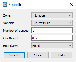
The dialog has the following options:
- Zone
-
Specify the zone to smooth from the drop-down. The zone should not intersect itself.
For a given plot type, the dimension of the zone must be less than or equal to the dimension of the plot type. That is, in 3D Cartesian plots, volume, surface and line zones may be smoothed, while in 2D Cartesian plots, volume zones cannot be smoothed.
- Variable
-
Select the variable to smooth. For line plots, the variable must be a dependent variable for an active mapping for that zone.
- Number of Passes
-
Specify the number of smoothing passes to perform. The default is 1. A greater number of passes results in greater smoothing, but takes more time.
- Coefficient
-
Specify the relaxation factor for each pass of smoothing. Enter a number between zero and one (exclusively). Large numbers flatten peaks and noise quickly. Small numbers smooth less each pass, rounding out peaks and valleys rather than eliminating them.
- Boundary
-
Select the boundary conditions by which to smooth from the Boundary drop-down.
- Fixed
-
The points at the boundary are not changed in value. For finite element data, only fixed boundary conditions may be used.
- First Order
-
The points at the boundary are smoothed based on the assumption that the first derivative normal to the boundary is constant. This will tend to cause contour lines of the smoothed variable to be perpendicular to the boundary.
- Second Order
-
The points at the boundary are smoothed based on the assumption that the second derivative normal to the boundary is constant. This option may overextrapolate derivatives at the boundary.
- Smooth
-
Click to perform smoothing. While the smoothing is underway, the progress is displayed in the status bar. A Stop button displayed in the status bar allows you to interrupt the operation.
Smoothing Method
Tecplot 360 uses the Jacobi method with the Coefficient used as a relaxation factor (always < 1, so it’s under-relaxed). For ordered zones, Tecplot 360 does this in generalized curvilinear coordinates, which has the effect of length- (or area- or volume-) weighting a node’s neighboring values. For the fixed boundary condition, boundary values remain unchanged. For first-order boundaries, the boundary values are relaxed toward the neighboring interior values, and for second-order boundaries, they are relaxed toward a constant slope (zero curvature) relative to the two neighboring interior points. For finite-element zones, Tecplot 360 relaxes each value toward the inverse-distance weighted average of its neighbors. Only the fixed boundary condition is available for FE zones.
Limitations of Smoothing
-
Finite element zones cannot be smoothed with anything other than Fixed boundary conditions.
-
Tecplot 360 uses the active frame’s axis assignments to determine the variables to use for the coordinates in the smoothing, and also to determine whether the smoothing should be done with XY Line, Polar, and 2D or 3D Cartesian plot types. Be sure to select the correct frame if you have multiple frames with different variable assignments for the same dataset.
-
Any axis scaling is ignored while smoothing.
-
For I-ordered or finite element line segment zones, the active frame can be in the XY Line, or 3D Cartesian plot types. In XY Line, the variable must be the dependent variable of one active mapping for that zone.
-
For IJ-ordered, finite element triangle, or finite element quadrilateral zones, the active frame can be a 2D or 3D Cartesian plot type, but you cannot smooth the variables assigned to the X and Y-axes in Cartesian.
-
For IJK-ordered, finite element tetrahedral, or finite element brick zones, the plot type must be 3D Cartesian, and you cannot smooth the variables assigned to the X, Y, and Z-axes. The IJK-mode is ignored. The zone is smoothed with respect to the entire 3D volume.
-
Smoothing does not extend across zone boundaries. If you use a boundary condition option other than Fixed (such that values along the zone boundary change), contour lines can be discontinuous at the zone boundaries.
-
Smoothing is performed on all nodes of a zone, and disregards value blanking.
Fourier Transform
The Fourier transform feature () allows you to transform one-dimensional ordered linear data into the frequency domain. One or more dependent variables in the data set are taken to be a representation of some function of a single independent variable, such as time, and this function is decomposed into its constituent sine waves. Variables are added to the data set to indicate these waves' frequency in Hertz, phase, and amplitude in each selected zone, and an XY of the resulting amplitudes is created in a new frame.
The dependent variables for a Fourier transform must be single-valued. The independent variable domain need not be constantly spaced; data will be resampled linearly if necessary.
The resulting frequency, amplitude, and phase variables (three for each dependent variable) are stored in Fourier transform result zones, one for each source zone. The result zones are given the name "Fourier Transform" followed by text indicating the source zone, independent variable, and window function used to calculate them. Result zones are assigned new time strands using the same groupings as the source zones if they belong to time stands; otherwise the resulting zones are static.
The result variables in the result zone are given the names Frequency, Amplitude and Phase followed by text indicating the dependent variable involved in the calculation. If the independent variable is non-uniform, Frequency is a uniform interpolation of the original data.
Newly-created zones are assigned passive variables for all variables that previously existed in the dataset, and all previously-existing zones are assigned passive variables for all new variables created by the Fourier transform.
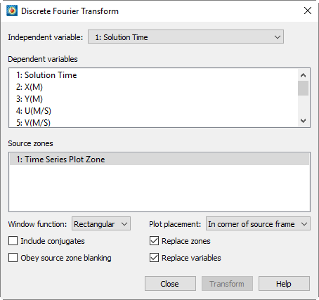
- Independent Variable
-
The variable used as the frequency domain. If this variable’s spacing is non-uniform, this variable is used in conjunction with each dependent variable for interpolation to create a uniform frequency for the Fourier transform.
- Dependent Variables
-
Choose the dependent variables to be transformed. Each will appear on the resulting XY plot as its own linemap.
- Source Zones
-
Choose the zones for which the transform should be calculated.
- Window Function
-
A function applied to the dependent variables before performing the transform (but after interpolation) to taper the data. Rectangular, triangular, Hann, and Hamming filters are provided.
- Plot Placement
-
Where to initially place the result plot of the transform showing the distribution of frequencies in the data. The plot can be moved and resized as desired afterward.
- In corner of source frame
-
A new frame is created for the frequency plot in the upper right corner of the frame containing the data being transformed.
- Tile with existing frames
-
All frames, including the new one, are adjusted to the same size and arranged on the paper in a grid.
- Include Conjugates
-
For purely real numbers, fully half of the results of the Fourier transform are conjugates (values with the same real part but opposite imaginary parts, which behave identically in situations where a real number is required). Toggling-off this option will allow the transform to be performed approximately twice as fast. as only one conjugate is calculated.
- Obey Source Zone Blanking
-
If value blanking is active and this option is toggled-on, value blanking is applied to the values of both independent and dependent variables before interpolation is performed. If data values eliminated by blanking cause the data to be non-uniform, the values are interpolated appropriately. All blanked data values up to the first non-blanked value, and all blanked data values after the last non-blanked value, are ignored, providing a way to constrain the domain of the transform.
- Replace Zones/Variables by Name
-
If either or both are toggled-on, the results of the transform are stored in existing result zones and/or variables, based on their names, if such zones and/or variables exist. Otherwise, new result zones and/or variables are created.
You may also access this feature by right-clicking a line map and choosing Fourier Transform from the context menu. In this case, the line map you click defines the independent and dependent variable used. All other settings are taken from last values entered in the dialog; the dialog does not appear.
Axial Rotation
The Axial Rotation dialog, available from the submenu of the menu, allows you to rotate one or more 2D or 3D zones using the right-hand rule. The variables rotated are the spatial variables (X, Y, and, for 3D zones, Z) and the vector variables assigned using . For 3D zones, you may also choose the axis of rotation.
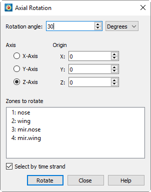
The Axial Rotation dialog has the following options:
- Rotation Angle
-
The angle by which the data should be rotated. May be specified in degrees or radians using the drop-down menu to the right of the entry field.
- Axis
-
For 3D zones, choose the axis around which rotation should occur. Not available for 2D zones, which are always rotated about a notional axis perpendicular to the zone.
- Origin
-
For rotation around a point other than (0, 0) or (0, 0, 0), enter the location of the origin using the X, Y, and (for 3D zones) Z fields.
- Zones to Rotate
-
Click, Control-click, and/or Shift-click in the zone list to select one or more zones.
Select by For transient data, if this checkbox is toggled on, the zones in the Zones to Rotate list are grouped by time strand, so that selecting a zone selects all the zones in that time strand.
Using a macro, it is possible to
rotate around arbitrary axes rather than just X, Y, and Z, and to
specify exactly which variables, if any, should be rotated as spatial
variables and which as vector variables, including no spatial variables
at all, or multiple vector variables. See $!ROTATEDATA in the Scripting Guide.
|
Zone Creation
The submenu of the menu allows you to add data to your plot. The menu has the following options:
Rectangular Zone Creation
Creating a rectangular zone is often the first step in interpolating irregular data into an ordered grid
Tecplot 360 allows you to create a new ordered rectangular zone with the dimensions in the I, J and K-directions you specify. This is done either with the tool (only) or the dialog. The zone that you create has the same number of variables as other zones in the dataset.
To create a rectangular zone, select from the menu.
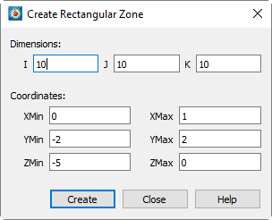
The dialog has the following options:
- Dimensions
-
Enter the number of data points in the I, J and K-directions.
-
To create an I-ordered zone, enter 1 for both the J and K-dimensions.
-
To create an IJ-ordered zone, enter 1 for the K-dimension. The z-axis variable will equal
ZMinthroughout the created zone. -
To create an IJK-ordered zone, enter a K-dimension greater than one.
-
- Coordinates
-
Enter the start and end points of the physical coordinates (X,Y and Z).
- Create
-
Select the [Create] button to create the zone.
Tecplot 360 uniformly distributes the data points in the I, J and K directions. Any variable not assigned to an axis is set to zero.
By using the dialog under the menu, you can modify the X, Y, and Z-coordinates, and the values of the other variables as well, by using equations or Equation files. See Data Alteration through Equations.
Circular or Cylindrical Zone Creation
Tecplot 360 allows you to create a new ordered circular or cylindrical zone with the dimensions in the I, J, and K-directions you specify. The I-dimension determines the number of points on each radius of the zones. The J-dimension determines the number of points around the circumference. The K-dimension determines the number of layers in the zone, creating a cylinder.
You create a circular or cylindrical zone with the dialog (accessed via , or with the tool (only). The zone that you create has the same number of variables as other zones in the dataset.
If you have no current dataset, Tecplot 360 creates one with two or three variables, depending on the K-dimension. If you specify , the dataset is created as IJ-ordered, and has two variables. If you specify , the dataset is created as IJK-ordered, and has three variables.
To create a circular zone select from the menu.
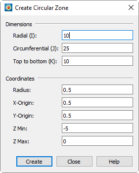
The dialog has the following options:
- Dimensions
-
Enter the dimensions of your circular zone:
- Radial (I)
-
Specify the number of points the radial direction (I)
- Circumferential (J)
-
Specify the number of points in the circumferential direction (J)
- Top to Bottom (K)
-
Specify the number of points for the height of the cylinder (K). Set K equal to one to create a circular zone.
- Coordinates
-
- Radius
-
Enter the length of the radius.
- X-Origin and Y-Origin
-
Enter the coordinates for the zone center
- ZMin and ZMax
-
Enter the minimum and maximum Z-coordinates. For a circular zone (where K=1), the Z variable is set to ZMin for all points.
- Create
-
Select the button to create the zone.
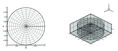
For IJ-ordered, Tecplot 360 creates a zone in which I-circles are connected by J-radial lines. For 3D (, Tecplot 360 creates a K-layered cylindrical zone having I-circles connected by J-radial planes. All other variables are set to zero These two scenarios are shown below
Using the option from the menu, you can modify the X-, Y-, and Z-coordinates, and the values of the other variables as well, by using equations or equation files. See Data Alteration through Equations.
Zone Duplication
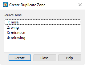
To create a full duplicate of one or more existing zones, select from the menu. In the dialog, select the source zone(s). Each duplicate zone has the same name as its source zone.
| After a zone is duplicated, all variables in the newly created zone(s) will be shared with their corresponding source zone(s). |
Mirror Zone Creation
To create a duplicate zone that is the mirror image of an existing zone, select from the menu.
| You can only create mirrored zones along one of the standard axes (2D) or the plane determined by any two axes (3D). |
The dialog has the following options:
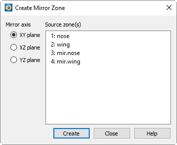
- Source Zone(s)
-
Select the Sources Zone(s).
- Mirror Axis
-
Specify the axis () or axis plane (3D) to mirror about.
- Create
-
Select the [Create] button to create the zone.
Each mirror zone has a name of the form "Mirror of zone sourcezone", where sourcezone is the number of the zone from which the mirrored zone was created.
| The variables in the newly created zone(s) are shared with their corresponding source zone(s), except for the coordinate and velocity normal to the symmetry plane. |
Axial Duplication
The Axial Duplication dialog, available from the submenu of the menu, allows you to create sucessively-rotated duplicates of one or more 2D or 3D zones using the right-hand rule. For example, if your data set contains a simulation of one blade of a turbine, and there are thirty blades in the full turbine, you can create 29 duplicates, each rotated twelve degrees from the previous, to be able to visualize the entire turbine.
The variables rotated are the spatial variables (X, Y, and, for 3D zones, Z) and the vector variables assigned using . For 3D zones, you may also choose the axis of rotation. Streamtraces are not duplicated; place streamtraces after zone duplication.
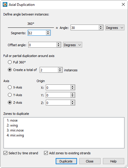
The Axial Duplication dialog has the following options:
- Define Angle Between Instances
-
Contains two interdependent fields, Angle and Segments, which are used to specify how many duplicates are in a full 360° rotation of the zone.
The number of segments is determined by dividing the angle into 360,° and the angle is calculated by dividing the number of segments into 360°. Editing one automatically updates the other. You may choose to specify (or calculate) the angle in ethier degrees or radians.
- Offset Angle
-
The additional amount by which the first duplicate should be rotated; may be specified in degrees or radians. For example, if you specify an angle between instances of 20° and an offset of 40°, the first duplicate will be made at 60°, the second at 80°, the third at 100°, and so on.
This field may be used, for instance, when you have already created some duplicates and want to create additional duplicates that do not overlap the ones you have already created. In the example just given of angle 20° and offset 40°, perhaps you have already created two duplicates (at 20'° and 40°) and wish to create additional duplicates. In this case, offset of 40° specifies that the last existing duplicate is at 40° and that new duplicates should be created in the next "slot" beyond that, at 60°.
- Full or Partial Duplication
-
Choose to create as many new zones as are necessary for a full rotation by choosing Full 360° (this will result in the number of duplicates entered or calculated in the , less the original zone(s) being duplicated) or create a specified number of rotated duplicates.
- Axis
-
For 3D zones, choose the axis around which rotation should occur. Not available for 2D zones, which are always rotated about a notional axis perpendicular to the zone.
- Origin
-
For rotation around a point other than (0, 0) or (0, 0, 0), enter the location of the origin using the X, Y, and (for 3D zones) Z fields.
- Zones to Duplicate
-
Click, Control-click, and/or Shift-click in the zone list to select one or more zones.
- Select by Time Strand
-
For transient data, if this checkbox is toggled on, the zones in the Zones to Duplicate list are grouped by time strand, so that selecting a zone selects all the zones in that time strand
- Add Zones to Existing Strands
-
For transient data, adds the duplicate zones to the same time strand as the original zones if toggled on. Otherwise, the duplicate zones are assigned new strand IDs if the soruce zones belonged to strands, otherwise they are made static.
Using a macro, it is possible to
rotate around arbitrary axes rather than just X, Y, and Z, and to
specify exactly which variables, if any, should be rotated as spatial
variables and which as vector variables, including no spatial variables
at all, or multiple vector variables. See $!AXIALDUPLICATE in the
Scripting Guide.
|
Data Extraction from an Existing Zone
You may create new zones by extracting (or interpolating) data from existing zones in a number of ways. Derived objects, such as contour lines, FE-boundaries, iso-surfaces, slices, or streamtraces may be extracted to be independent zones. You may also extract data using a specified slice plane, discrete points, points from a polyline, or points from a geometry.
The procedures for extracting derived objects are discussed in the chapters related to those objects. For details see Contour Layer, Streamtrace Extraction as Zones, and Iso-Surface Extraction. Extracting slices, both derived and arbitrarily defined, is described in Extracting Slices to Zones.
Subzone Extraction
To create a subzone of an existing ordered zone, select from the menu.
| Subzone extraction is available for ordered zones only. |
The dialog has the following options:
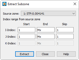
- Source Zone
-
Select the source zone (ordered zones only).
- Index Range from Source Zone
-
Specify the desired subzone as a range of I, J, and K-indices. You may use the special value
0orMxto indicate the maximum of that index, and the valuesMx-1to represent one index less than the maximum,Mx-2for two less than the maximum, and so forth. - Extract
-
Select the button to create the zone. Each extracted subzone is given the name "Subzone."
Data Point Extraction
You may create an I-ordered zone by extracting data points from the current dataset along a polyline that lies within the edges of a zone with connectivity. To extract points along a polyline:
-
If necessary, create the polyline geometry using the
 polyline tool. Click each of the points in the polyline, then
double-click the last point (or press Escape) to finish the polyline.
You may also extract points along an already-existing polyline.
 -
Right-click the polyline geometry in the workspace and choose Extract Points from the context menu to open the dialog.
-
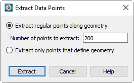
Use the dialog to control how data points are extracted. The dialog has the following options:
- Extract regular points along geometry
-
Select this option to extract the specified number of points distributed uniformly along the geometry.
- Number of points to extract
-
Enter the number of points to extract. This field is available only if you are extracting regular points along a geometry.
- Extract only points which define geometry
-
Select this option to extract only the endpoints of the segments in the geometry.
Any necessary interpolation is performed using the same method used in probing. The spatial interpolation method is piecewise-linear by default. Cells are, in effect, divided by adding nodes at their center and face centers, until all cell pieces are tetrahedral. The extra nodes are calculated by arithmetically averaging the variable values at all nodes (for the cell-center node) or all face nodes (for the face-center nodes). Within each of these sub-cells, variables are interpolated linearly.
From triangular faces, linear interpolation is used to determine the value of the extracted points. On quadrilateral faces, a point of the center of mass of the quadrilateral is created and assigned a value equal to the average of the four corners. The surface is then broken down into four triangles using this center point and the four corners, and the extracted point value is interpolated linearly on the face of the triangle that surrounds it.
If a surface utilizes cell-centered values, the nodal values at the corners are interpolated, then the extracted points are interpolated from those nodal values.
Volume interpolation, piece-wise by default, calculates to first-order accuracy. For second-order accuracy (tri-linear interpolation), add the following line to your tecplot.cfg file:
$!INTERFACE DATA {VOLUMECELLINTEROPLATIONMODE = TRILINEAR} -
If you created a new polyline for the extraction operation, you may wish to delete it by again right-clicking it, then choosing from the context menu.
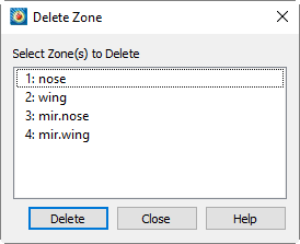
Zone Deletion
In any dataset with more than one zone, you can delete any unwanted zones. To delete a zone, select from the menu. You cannot delete all zones; if you attempt to delete all zones, the lowest numbered zone is not deleted.
Variable Deletion
To delete a variable, select from the menu. The dialog is shown below.
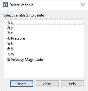
When deleting a variable, keep in mind that deleting a variable removes it from all zones. You cannot delete a variable used in a Calculate-on-demand function. See Calculate-on-demand Variables.
Data Interpolation
In Tecplot 360, interpolation refers to assigning new values for the variables at data points in a zone based on the data point values in another zone (or set of zones).
For example, you may have a set of data points in an I-ordered zone that are distributed randomly in the XY-plane. This type of data is sometimes referred to as unordered, ungridded, or random data. In Tecplot 360, it is referred to as irregular data. Using data in this form, you can create mesh plots and scatter plots, but you cannot create contour plots, light-source shading, or streamtraces.
In Tecplot 360, you can interpolate the irregular I-ordered data onto an IJ-ordered mesh, and then create contour plots and other types of field plots with the interpolated data. You can also interpolate your 3D, I-ordered irregular data into an IJK-ordered zone and create 3D volume plots from the IJK-ordered zone. You can even interpolate to a finite element zone.
The accuracy of the interpolation will depend on your data, the density of the destination grid, how well the grid fits the area of your unorganized zone and the settings used for interpolation.
There are three types of interpolation available:
- Linear Interpolation
-
Interpolate using linear interpolation from a set of finite element, IJ-ordered, or IJK-ordered zones to one zone.
- Inverse-Distance Interpolation
-
Interpolate using an inverse-distance weighting from a set of zones to one zone.
- Kriging
-
Interpolate using Kriging from a set of zones to one zone.
Linear Interpolation
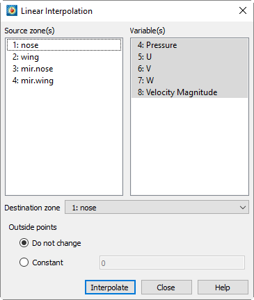
Use the dialog to interpolate data from one or more ordered or finite element zones onto a destination zone. Irregular I-ordered data cannot be used for the source zones in linear interpolation; you may be able to first create a finite element zone from an irregular, I-ordered zone by using triangulation. (See Irregular Data Point Triangulation.)
Linear interpolation finds the values in the destination zone based on their location within the cells of the source zones. The value is linearly interpolated to the destination data points using only the data points at the vertices of the cell (or element) in the source zone(s).
To perform linear interpolation:
-
Read the dataset to be interpolated into Tecplot 360 (the source data).
-
Read in or create the zone onto which the data is to be interpolated (the destination zone).
-
From the menu, choose .
-
From the dialog, select the zones to be interpolated from those listed in the scrolled list.
-
Select which variables are to be interpolated from those listed in the scrolled list.
-
Select the destination zone into which to interpolate. Existing values in the destination zone will be overwritten.
-
- Optionally, choose how to treat points that lie outside the source-zone data field. You have two options:
-
- Preserves the values of points outside the data field. is appropriate in cases where you are using one interpolation algorithm inside the data field, and another outside.
-
- Sets all points outside the data field to a constant value that you specify.
-
-
Click the [Interpolate] button to perform the interpolation.
-
While the interpolation is proceeding, a working dialog appears showing the progress of the interpolation
| If you select [Cancel] during the interpolation process, the interpolation is terminated prematurely. The destination zone will be left in an indeterminate state, and you should redo the interpolation. |
Inverse-Distance Interpolation
Inverse-distance interpolation averages the values at the data points from one set of zones (the source zones) to the data points in another zone (the destination zone). The average is weighted by a function of the distance between each source data point to the destination data point. The closer a source data point is to the destination data point, the greater its value is weighted.
In many cases, the source zone is an irregular dataset—an I-ordered set of data points without any mesh structure (a list of points). Inverse-distance interpolation may be used to create a 3D surface or a 3D volume field plots of irregular data. The destination zone can, for example, be a circular or rectangular zone created within Tecplot 360 Zone Creation).
To perform inverse-distance interpolation in Tecplot 360, use the following steps:
-
Read the dataset to be interpolated into Tecplot 360 (the source data).
-
Read in or create the zone onto which the data is to be interpolated (the destination zone).
-
From the menu, choose .
-
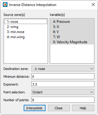
From the dialog, select the zones to be interpolated from those listed in the list.
-
Select which variables are to be interpolated from those listed in the list.
-
Select the into which to interpolate. Existing values in the destination zone will be overwritten.
-
[OPTIONAL] Enter the minimum distance used for the inverse-distance weighting in the text field. Source data points which are closer to a destination data point than this minimum distance are weighted as if they were at the minimum distance. This tends to reduce the peaking and plateauing of the interpolated data near the source data points.
-
[OPTIONAL] Enter the exponent for the inverse-distance weighting in the text field.
The exponent should be set between 2 and 5. The algorithm is speed-optimized for an exponent of 4, although in many cases, the interpolation looks better with an exponent of 3.5. -
[OPTIONAL] Select the method used for determining which source points to consider for each destination point from the drop-down. There are three available methods, as follows:
- Nearest N
-
For each point in the destination zone, consider only the closest n points to the destination point. These n points can come from any of the source zones. This option may speed up processing if n is significantly smaller than the entire number of source points.
- Octant
-
Like above, except the
npoints are selected by coordinate-system octants. Thenpoints are selected so they are distributed as evenly as possible throughout the eight octants. This reduces the chances of using source points which are all on one side of the destination point. - All
-
Consider all points in the source zone(s) for each point in the destination zone.
-
Click to perform the interpolation.
| If you select the button during the interpolation process, the interpolation is terminated prematurely. The destination zone will be left in an indeterminate state, and you should redo the interpolation. |
Inverse-distance interpolation ignores the IJK-mode of IJK-ordered zones. All data points in both the source and destination zones are used in the interpolation.
| Tecplot 360 uses the active frame’s axis assignments to determine the variables to use for coordinates in interpolation. However, axis scaling is ignored. |
The Inverse-Distance Algorithm
The algorithm used for inverse-distance interpolation is simple. The value of a variable at a data point in the destination zone is calculated as a function of the selected data points in the source zone (as defined in the drop-down, accessed via ).
The value at each source zone data point is weighted by the inverse of the distance between the source data point and the destination data point (raised to a power) as shown below:
where and are the values of the variables at the destination point and the source point, respectively, and is the weighting function defined as:
D in the equation above is the distance between the source
point and the destination point or the minimum distance specified in the
dialog, whichever is greater. E is the exponent specified
in the text field.
Smoothing may improve the data created by inverse-distance interpolation. Smoothing adjusts the values at data points toward the average of the values at neighboring data points, removing peaks, plateaus, and noise from the data. See Data Smoothing for information on smoothing.
|
Kriging and Inverse Distance Interpolation Improvements
For better results with 3D data, try changing the range of your
Z-variable to one similar to the X-range the Y-range. Also, set Zero
Value to 0.05.
|
Kriging
Kriging is a more complex form of interpolation than inverse-distance. It generally produces superior results to the inverse-distance algorithm but requires more computer memory and time.
To perform kriging in Tecplot 360, perform the following steps:
-
Read the dataset to be interpolated into Tecplot 360 (the source data).
-
Read in or create the zone onto which the data is to be interpolated (the destination zone).
-
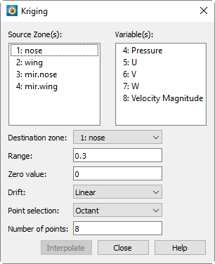
From the menu, choose
-
From the dialog, select the zones to be interpolated from those listed in the scrolled list.
Tecplot 360 uses the active frame’s axis assignments to determine the variables to use for coordinates in kriging. However, any axis scaling is ignored. -
Select which variables are to be interpolated from those listed in the scrolled list.
-
Select the destination zone into which to interpolate. Existing values in the destination zone will be overwritten.
-
In the text field, optionally enter the distance beyond which source points become insignificant for the kriging. The value is stated as the fraction of the length of the diagonal of the box which contains the data points. A range of zero means that any point not coincident with the destination point is statistically insignificant; a range of one means that every point in the dataset is statistically significant for each point. In general, values between 0.2 and 0.5 should be used.
-
In the text field, optionally enter the semi-variance at each source data point on a normalized scale from zero to one. Semi-variance is the certainty of the value at a data point. A value of zero means that the values at the source points are exact. Greater values mean the values at the source points have some uncertainty or noise. Zero is usually a good number for the zero value, and it causes the interpolated data to fit closely to all the source data points. Increasing the zero value results in smoother interpolated values that fit increasingly more to the average of the source data.
-
Select the overall trend for the data in the drop-down. This can be (default), or .
If the is set to Linear or Quadratic, Tecplot 360 requires that the points selected be non-collinear (non-coplanar in 3D). To avoid this limitation, set to None. Alternatively, you can eliminate coincident points by Irregular Data Point Triangulation before you interpolate. -
Select the method used for determining which source points to consider for each destination point from the drop-down. There are three available methods, as follows:
- Nearest N
-
For each point in the destination zone, consider only the closest n points to the destination point. These n points can come from any of the source zones.
- Octant (default)
-
Like Nearest N above, except the n points are selected by coordinate-system octants. The n points are selected so they are distributed as evenly as possible throughout the eight octants. This reduces the chances of using source points which are all on one side of the destination point.
- All
-
Consider all points in the source zone(s) for each point in the destination zone. In general, you should not use the All option unless you have very few source points
The option is very important for kriging, because kriging involves the computationally expensive inversion and multiplication of matrices. The computational time and memory requirements increase rapidly as the number of selected source data points increases. -
Click to begin kriging. While kriging is proceeding, a progress bar appears in the status bar, along with a Stop button that can be clicked to interrupt the operation.
| If you interrupt the kriging process, the destination zone is left in an indeterminate state, and you should redo the kriging or delete the destination zone. |
The Kriging Algorithm
For a detailed discussion of the kriging algorithm refer to: Davis, J. C., Statistics and Data Analysis in Geology, Second Edition, John Wiley & Sons, New York, 1973, 1986.
| Kriging and Inverse Distance Interpolation Improvements#: For better results with 3D data, try changing the range of your Z-variable to one similar to the X-range the Y-range. Also, set Zero Value to 0.05. |
Irregular Data Point Triangulation
Triangulation is a process that connects data points to form triangles. You can use triangulation to convert irregular I-ordered datasets into a finite element surface zone. Triangulation is one of the two options for creating field plots from irregular data. The other is interpolation, discussed in Data Interpolation. Triangulation preserves the accuracy of the data by creating a finite element surface zone with the source data points as nodes and a set of triangle elements. Triangulation works best for irregular data.
To triangulate 2D data, make sure your plot is in 2D Cartesian mode and select from the menu. The dialog has the following options:
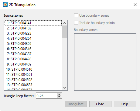
- Source Zone(s)
-
Select the zone or zones to triangulate from the list.
- Use Boundary Zone(s)
-
Toggle-on to specify a boundary zone for the triangulation. Select the boundary zone or zones from the list. The boundary zones define the boundaries in the triangulation region. If you do not include boundary zones, Tecplot 360 assumes the data points lie within a convex polygon and that all points in the interior can be connected.
- Include Boundary Points
-
Toggle-on to include the points in the boundary zones in the triangulated zone.
- Triangle Keep Factor
-
This factor is used to define which triangles on the outside of the triangulated zone are "bad" and not included in the triangulation.
At the completion of triangulation, Tecplot 360 attempts to remove bad triangles from the outside of the triangulation. The keep factor is a description of the shape of the triangle between zero (three collinear points) and 1.0 (an equilateral triangle). Typical settings are values between 0.1 and 0.3; settings above 0.5 are not permitted. Bad triangles will not be removed if removing the triangle strands a data point.
- Triangulate
-
Click the button to perform the triangulation.
After triangulating your data, you can use the resulting finite element surface zone to create plots. Generally, you turn off the original zone(s) and plot the new zone only, but you can, for example, plot a scatter plot of the original zone(s) along with the contours of the new zone.
Data Spreadsheet
All ordered and finite element data can be viewed using Tecplot 360’s data spreadsheet (accessed via ). The data may be modified within the spreadsheet in order to change the plots Tecplot 360 produces.
| Changes to the spreadsheet do not immediately alter the original data file stored on disk. However, saving the plot of altered data as a layout file will save the changes in the data journal. You have the option of overwriting your original data file or creating a new file with the altered data. |
The spreadsheet displays Tecplot 360’s data differently depending on the type of zone being examined. An example of the dialog for a finite element zone is shown here; note the X, Y, and Z variables.
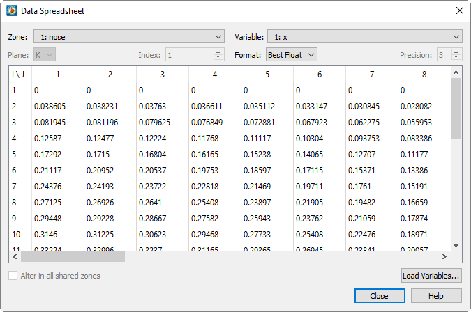
I-ordered and finite element datasets are displayed with each zone’s variable displayed in a column. IJ-ordered datasets are displayed in the spreadsheet with I along the rows and J along the columns. IJK-ordered datasets are displayed one plane at a time: selecting the K-plane displays I along the rows and J along the columns, selecting the J-plane displays I along the rows and K along the columns, and selecting the I-plane displays J along the rows and K along the columns. With IJK-ordered data, the slice of interest can be selected by entering a specific index or using the up and down arrows provided.
If a variable is not needed in your plot, it may not currently be loaded into memory. In this case, "Not Loaded" is displayed in every cell of that variable’s column. Using the variable in your plot will cause it to be loaded. Click the button to open the Load Variable dialog and load any variables you wish to view and edit in the spreadsheet.
To change the data spreadsheet’s display format, select the desired format (Integer, Float, Exponent, or Best Float) from the Format drop-down menu. When Float or Exponent is selected, you may also specify the precision in the Precision field. These options do not affect the actual data, only how it is displayed.
To modify data:
-
In the dialog, select a zone and variable to modify. Use the menu at the top of the dialog to choose the zone, then find the column representing the desired variable.
-
If the variable is shared with another zone or zones, the toggle is enabled. Select this toggle to keep the variable shared as you modify data, propagating changes to the other zones that share the variable. If this toggle is not selected, the variable will be changed in the selected zone and no longer shared with any other zones. See also Data Sharing.
-
Select the value of interest from the spreadsheet by finding its row. This will highlight and expand the value to its full precision.
-
To replace the highlighted value, simply enter the new value. The value is instantly replaced with the new digits entered.
-
To modify only a few digits from a highlighted value, double-click the cell to switch to edit mode. Click again or use the arrow keys to position the edit cursor at the desired position. Make any desired modifications to the existing value such as inserting or deleting digits.
-
To undo a modification of a given cell before you have committed it, press
Escape. To commit a modification, pressEnter,Tab, orShift-Tabto move to the next cell, or simply select on another cell.
$!INTERFACE DATA {DERIVATIVEBOUNDARY = method} setting the configuration file tecplot.cfg to select the method to use. Set method to SIMPLE or COMPLEX.