Viewing XY Data
Data Spreadsheet
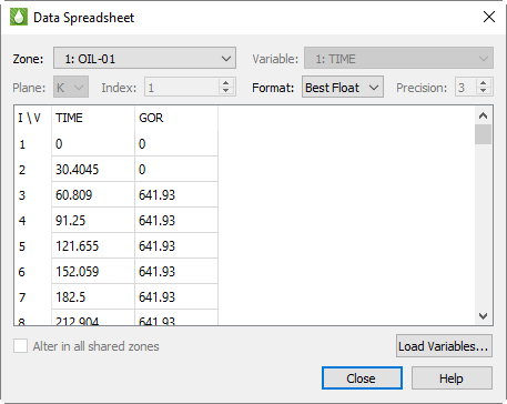
You can view loaded XY data in the Data Spreadsheet dialog by choosing from the menu. In this dialog, you can edit data, adjust the formatting of the displayed data, copy the data to your operating system’s clipboard, and paste it into another program.
The Data Spreadsheet dialog displays the entities and variables selected in the sidebar: the entity appears in the menu, and the variables currently chosen for that entity appear in the table below.
| You must have at least one entity and one variable selected in the sidebar in order to open the Data Spreadsheet dialog. |
Spreadsheet Formatting
Using the formatting controls at the top of the Data Spreadsheet dialog, you can change the format of the displayed data without changing your data file(s) or the appearance of your plot.
-
Format Choose a number format from the Format menu in the dialog that best represents the data. You can choose from displaying the data in Integer, Float, Exponent, or Best Float form.
-
Precision If you have Float or Exponent chosen as the Format, you can specify the number of places displayed to the right of the decimal.
If some values are too wide to fit in their column, the width of the column may be adjusted by dragging the divider lines in the heading.
Editing Spreadsheet Data
To edit any displayed value, double-click it, type the new value, and press Enter. Changes made here are applied only to the plot; they do not affect the underlying data set. If you change the plot type, your changes will be lost.
Periodic Production Rates
You can calculate Production rates on weekly, biweekly, monthly, quarterly, and annual intervals using cumulative variables from the active XY dataset or from all loaded datasets. To use this feature, choose .
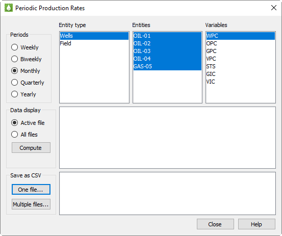
In the Periodic Production Rates dialog, you first select a time period. You may then select one Entity Type. The supported entity types are Wells, Field, Groups/Areas, Regions, and User Groups. Each entity type is displayed in the list only if it is present in the dataset. After you select the entity type, the available entities and variables are displayed. You can then select one or more entities and/or variables.
| To be displayed in the variable list, a variable must be cumulative (never decreasing in value with increasing time) and nonzero across all entities. |
Finally, if you have loaded more than one XY dataset, you can choose to have the results displayed for the active file or for all files.
Displaying Results
Once the desired selections have been made, click Compute to show the calculated data in the dialog.
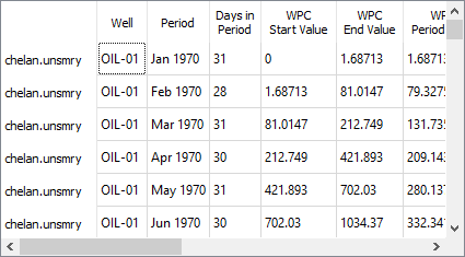
After you click Compute, the results are displayed in a table like the one above. The following columns are included:
-
Dataset name - The first column shows the name of the dataset from which each row’s result was calculated. If you are displaying results from multiple datasets, the number of the dataset (starting with 1) and a colon appear before the name of the dataset.
-
Entity - The title of this column changes depending on the entity type selected. In the example above, it is Wells. This column identifies the specific entity for which the row’s result was calculated.
-
Period - The period for which this row was calculated.
-
Days in Period - The number of days the period spans. Often, this will show the total days in the selected period (e.g., 28, 29, 30, or 31 days for a monthly period), but at the beginning or end of the data’s time range, it may be less, which implies that data for only part of that time period is available.
The following columns appear next, repeating once for each variable. The name of each column is prefaced by the variable name (for example, "OPC Start Value"). For each variable, the following values are displayed:
-
Start Value - The beginning cumulative variable value in the time period. If data aren’t available at the start time, it’s linearly interpolated from surrounding values.
-
End Value - The ending cumulative variable value in the time period. If data aren’t available at the end time, it’s linearly interpolated from surrounding values.
-
Period Rate - The difference between the ending and beginning cumulative variable value in the time period.
-
Avg Daily Rate - Period Rate divided by Days in Period.
-
Prod Days - Number of days in the period during which the cumulative variable increased, which implies production.
-
Avg Prod Rate - Period Rate divided by Prod Days.
After the above columns for the selected variables, the Start Day column is displayed. This is the Excel serial number (i.e., the number of days since January 1, 1900) of the start day in the period. These values can be used to show dates on the axis label for plots generated in Microsoft Excel and other spreadsheet programs that support this format.
Saving Results to CSV
To easily use this information with other programs, save the results as a CSV file. Click either the One File or the Multiple Files button. The two options behave as follows:
-
One File - You are prompted for a location and a file name. All the results displayed in the table (whether for one dataset or for all loaded datasets) are saved to the specified file.
-
Multiple Files - For each dataset loaded, a CSV file is created in the directory that contains the original data file. The files are automatically named with the original data file name, the entity type, and the selected period (for example, spe9a_xyp_WELLS_Monthly.csv). If CSV files already exist with these names, they are silently overwritten.
Tecplot RS reminds you of this behavior when you click the Multiple Files button.
The columns in the exported CSV file are as previously described in Displaying Results.