Basic Grid Plots
You can choose the type of grid display (2D or 3D) in the menu, or by using the small menu at the bottom of the sidebar.
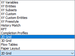
2D Grid Plots display one plane (layer) of grid cells at a time. You can choose which plane to plot by specifying both the view (I, J, or K) and the plane index. Radial grids can also display the views at constant R or Theta values.
3D Grid Plots show the entire reservoir grid in an orthogonal or perspective view. The initial orientation of the view is preset, but you can easily rotate, zoom, or translate the view.
2D Grid Plots
To view a 2D plot of a loaded grid file, choose from the menu. The plot will change and the 2D Grid Plot Controls sidebar will appear.
You can un-dock the Plot Controls sidebar by dragging its title bar to a new position. To put the Plot Controls back on the side of the workspace, double-click on its title bar (the region that displays the plot type). Or you can drag its title bar to either side of the workspace and let go, and it will snap into place.
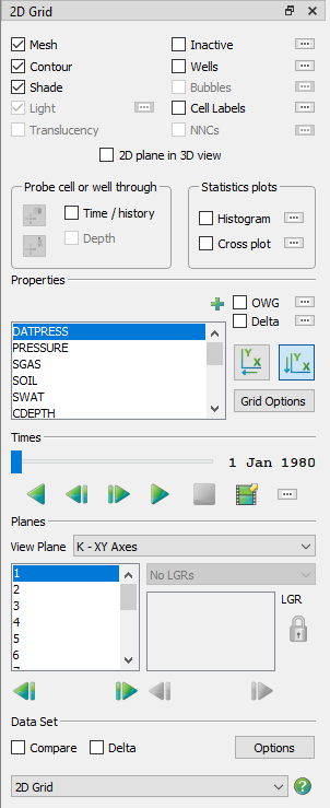
The sidebar for 2D Grid plots has the options described following.
-
Mesh Layer This toggle turns on or off the grid mesh.
-
Contour Layer The Contour toggle controls display of the flooded contours, either as a solid color in each cell or bands of constant color.
-
Connect When displaying wells, the Connect toggle turns on and off the lines connecting the well nodes.
-
Shade Layer You can control the Shade only when Contour is toggled-off. Use this toggle to turn on or off the surface shading, making the interior of the grid mesh visible or hidden.
-
Inactive Cells Toggle-on "Inactive" to display the inactive cells along with the active cells in your grid. If you have not loaded the inactive cells associated with the active grid, Tecplot RS will prompt you load them. See Loading Inactive Cells for details. See Inactive Cells for information on how to display solution data on inactive cells.
-
NNCs (2D Grid plots) Toggle-on this option to make Non-Neighbor Connections (NNCs) visible. Use the Details button to display the NNC dialog.
-
Wells Toggle-on "Wells" to display any wells in the current plot. The shape of the symbol indicates the type of well (producer, injector, and so forth). The Details button adjacent to Wells brings up the Wells dialog.
-
Bubble Plots Toggle-on "Bubbles" to show well data represented as bubbles on the well heads.
-
Cell Labels Toggle-on "Cell Labels" to include cell or well labels in your plot.
-
Time/History Toggling-on "Time/History" creates a new frame that you can use to display an XY line plot. You can choose to plot value versus time for a single cell in the grid or for a selected well. The current variables chosen in the XY Variables plot type determines the variables shown in the Time/History plots.
-
Depth If you include RFT data in your current XY data set, you can plot them in a manner similar to the Time/History plots by toggling-on "Depth". You can choose which variables to display by using the RFT Plots plot type.
-
Statstics Displays or hides a statistical plot, either a histogram or cross plot (only one of these plots may be visible). Choose Histogram or Cross Plot from the sidebar to choose which plot will be displayed and to set its options; for more details, see Statistical Plots.
-
2D Plane in 3D View Toggling-on "2D Plane in 3D" will convert the final frame of multi-frame plots to a 3D view. If you are in single-frame mode, it will switch the active frame to a 3D view. The 3D view works well for determining the location of the chosen plane(s) relative to the complete grid.
| To plot well data instead of cell data in your Time/History plot, select the well crosshair on the sidebar or hold down the Ctrl key and choose a well head or a cell containing a well. |
-
Variables The Variables box lists each variable that you can use for a contour plot. Time-dependent (dynamic) variables display first, followed by time-independent (static) variables. When you have a variable highlighted, each cell in the grid plot will display filled with a color representing the value of that variable at the chosen time.
-
Variable Display Controls Use the OWG option to create a ternary (red-green-blue) color map to color cells based on their combined saturations.
-
Time Delta Choosing "Delta" causes the contour display to reflect the variable value at a selected time, relative to the reference time step.
-
2D Grid Axis Orientation
 Two toggles buttons control whether to reverse the X and Y axes. These
settings connect to the View plane settings, so you can set reverse toggles
for the I plane independently of the K plane.
Two toggles buttons control whether to reverse the X and Y axes. These
settings connect to the View plane settings, so you can set reverse toggles
for the I plane independently of the K plane. -
Grid Options Click this button to bring up a dialog in which you can control many customizations of your grid plot, including loading inactive cells, translating and/or rotating your grid, and more.
-
Expanded List button Whenever you see the Plus button,
 next to a list in the sidebar
or a dialog, you can click this button to open an expanded version of the
list contents. To find an item in the list more easily, you can type
letters in the Filter field at the top of the list. Only items that include
those letters in that order will appear in the expanded list. For example,
to display only items with the word "well" in their name, type "well" into
the Filter field.
next to a list in the sidebar
or a dialog, you can click this button to open an expanded version of the
list contents. To find an item in the list more easily, you can type
letters in the Filter field at the top of the list. Only items that include
those letters in that order will appear in the expanded list. For example,
to display only items with the word "well" in their name, type "well" into
the Filter field.
-
-
Paging: Animation and Scrolling Controls The Times region of the sidebar allows you to choose a time step or animate the progression of a time-dependent variable. Use the slider to control time step.
-
Planes In the Planes region of the sidebar, use the Plane menu to choose logical planes (I, J, or K) to view and the physical plane (YZ, XZ, or XY) or logical plane (JK, IK or IJ) onto which it is projected. For example, choosing J(XZ) will plot only the data at the J-index highlighted in the box, with X as the horizontal axis and depth (Z) on the vertical axis.
When you are working with a radial grid, the list will include R and Theta views. When you make a change, the list of indexes in the box will reflect the new limits for that view (for example, you may have ten J planes but only three K planes).
-
Local Grid Refinement (LGR) The Local Grid Refinement (LGR) menu and box activate when an LGR intersects the selected plane from the global grid. The menu will show a list of the intersected LGR names. The box will show a list of planes which are part of the LGR selected in the menu.
Where an LGR exists, use the menu to select the LGR and the box to choose its index. In this manner you can switch from the coarse levels of the left-hand box to finer control.
Child LGRs appear indented relative to their parent LGR. You can “lock” the relationship between the parent and child LGRs, so that they update each other. To do this, click the Lock button next to the LGR. While the lock is “on”, choosing a parent grid plane will update the plane in the child grid, and changing the plane in a child grid will update the parent grid plane.
-
| By default, changing the plane in a child LGR grid will not update the parent grid plane. |
|
When multi-reservoir grids are loaded, there is an extra “placeholder” grid with the GLOBAL name, and its dimensions will be N x N x N, where N is the number of reservoirs. In the 2D grid controls, choosing the I, J, or K plane for the GLOBAL grid will actually choose the reservoir number. The LGR list will then be populated with the true grids for that reservoir. In the 2D Grid plot type, each reservoir is managed independently. This means, for example, that you can’t see K plane #5 in two different reservoirs. If this functionality is needed, use Inside View -IJK Slices in the 3D Grid plot type instead. |
3D Grid Plots
To view a 3D plot of a grid file, choose from the menu. The display of your plot will change to a 3D view and the Plot Controls sidebar will appear.
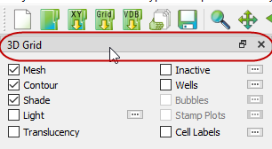
You can un-dock the Plot Controls sidebar by dragging its title bar to a new position. To put the Plot Controls back on the side of the workspace, double-click on its title bar (the region that displays the plot type). Or you can drag its title bar to either side of the workspace and let go, and it will snap into place.
The sidebar for 3D Grid plots has the options described following:
-
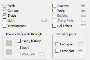
Mesh Layer This toggle turns on or off a mesh of lines on your plot.
-
Contour Layer The "Contour" toggle controls display of flooded contours.
-
Connect When you have "Wells" toggled-on, this toggle turns on and off the lines connecting the well nodes.
-
Shade Layer You can control the Shade only when Contour is toggled-off. Use this toggle to turn on or off the surface shading, making the interior of the grid mesh visible or hidden.
-
Lighting Layer (3D Grid plots only) Use this toggle to turn on and off light source shading. When on, shadows make it easier to visualize the shape of the 3D model and mute the colors.
-
Translucency Layer (3D Grid plots only) With "Translucency" toggled-on, the grid surface becomes translucent, making it possible to see the interior of the model.
-
Inactive Cells Toggle-on "Inactive" to display the inactive cells along with the active cells in your grid. If you have not loaded the inactive cells associated with the active grid, Tecplot RS will prompt you load them. See Loading Inactive Cells for details. See Inactive Cells for information on how to display solution data on inactive cells.
-
NNCs (2D Grid plots) Toggle-on this option to make Non-Neighbor Connections (NNCs) visible. Use the Details button to display the NNC dialog.
-
Wells Toggle-on "Wells" to display any wells in the current plot. The shape of the symbol indicates the type of well (producer, injector, and so forth). The Details button adjacent to Wells brings up the Wells dialog.
-
Bubble Plots Toggle-on "Bubbles" to show well data represented as bubbles on the well heads.
-
Cell Labels Toggle-on "Cell Labels" to include cell or well labels in your plot.
| The Light, Shade, and Translucency toggles are automatically set whenever you choose an option that would activate or deactivate a see-through grid. This includes turning on NNCs, Streamlines, and the Ghost option for inside views. |
-
Time/History Toggling-on "Time/History" creates a new frame that you can use to display an XY line plot. You can choose to plot value versus time for a single cell in the grid or for a selected well. The current variables chosen in the XY Variables plot type determines the variables shown in the Time/History plot. (To plot from a selected well, you must have the corresponding XY data loaded.) If you plot from a cell, Tecplot RS will use the variable currently selected in the 2D or 3D Grid plot to plot the variable versus time.
| To plot well data instead of cell data in your Time/History plot, hold down the Ctrl key and select a well head or a cell containing a well. |
-
Depth If you include RFT data in your current XY data set, you can plot them in a manner similar to the Time/History plots by toggling-on "Depth". You can choose which variables to display by using the RFT Plots plot type.
-
Well Path Creates an XY plot similar to the Time/history and Depth plots by toggling-on "Well Path". Only available in 3D Plots. Select the cell contianing a well to follow the values along the well path. Can be shown in distance along well path or vertical depth.
-
Statstics Displays or hides a statistical plot, either a histogram or cross plot (only one of these plots may be visible). Choose Histogram or Cross Plot from the sidebar to choose which plot will be displayed and to set its options; for more details, see Statistical Plots.
-
Variables The Variables box lists each variable that you can use for a contour plot. Time-dependent (dynamic) variables display first, followed by time-independent (static) variables. When you have a variable highlighted, each cell in the grid plot will display filled with a color representing the value of that variable at the chosen time.
-
OWG (Oil/Water/Gas) Saturation Plots Use the OWG option to create a ternary (red-green-blue) color map to color cells based on their combined saturations.
-
Time Delta Choosing "Delta" causes the contour display to reflect the variable value at a selected time, relative to the reference time step.
-
KSum Choose "KSum" to display the sum of the variable values in a column (all cells with matching I and J indexes) for all displayed layers.
-
KAvg Choose "KAvg" to display the average of the variable values in a column (all cells with matching I and J indexes) for all displayed layers.
-
Grid Options Click this button to bring up a dialog in which you can control many customizations of your grid plot, including loading inactive cells, translating and/or rotating your grid, and more.
-
Expanded List button Whenever you see the Plus button,
next to a list in the sidebar
or a dialog, you can click this button to open an expanded version of the
list contents. To find an item in the list more easily, you can type
letters in the Filter field at the top of the list. Only items that include
those letters in that order will appear in the expanded list. For example,
to display only items with the word "well" in their name, type "well" into
the Filter field.
-
-
Paging: Animation and Scrolling Controls The Times region of the sidebar allows you to choose a time step or animate the progression of a time-dependent variable. Use the slider to control time step.
-
Inside Views The Inside Views region of the sidebar provides options for displaying the grid solution.
| You can store a 3D view (rotation, center, and perspective) and quickly return to it later using the Save and Apply Custom 3D View options on the View menu. See Custom 3D View for more details. |
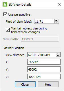
3D View Details
Use the 3D View Details dialog (accessed via the menu) to control a variety of parameters affecting the display of 3D Grid plots.
-
Use Perspective - Sets Tecplot RS’s projection type. If selected, Tecplot RS draws the current frame with perspective projection. If not selected, Tecplot RS draws the current frame with orthographic projection. (Range is 0.1 to 179.9.)
With orthographic projection, the shape of the objects is independent of distance. This is sometimes an "unrealistic" view, but it is often used for displaying physical objects when preserving the true lengths is important (such as drafting).
-
Field of View (deg) - Sets the amount of the plot (in terms of spherical arc) in front of the viewer that may be seen. Zooming in or out of a 3D perspective plot changes this number and the viewer’s position.
-
Maintain Object Size During Field of View Changes - If selected, Field of View changes result in the viewer’s position being moved so that approximately the same amount of the plane is visible after the change.
If not selected, Field of View changes do not change the viewer’s position and result in the entire plot appearing to grow or shrink.
-
View Width - Sets the amount of the plot (in X-axis units) in front of the viewer that may be seen. Zooming in or out of a 3D orthographic plot changes this number, but not the viewer’s position.
-
Viewer Position - Change the viewer’s relation to the image by resetting the X, Y, or Z-location, or by changing the view distance.
Common Controls
2D and 3D grid plots in Tecplot RS share many powerful features, especially those controlled by the sidebar. You can use the following controls on both 2D Grid Plots and 3D Grid Plots:
Time Options
Use the Time Options dialog to specify a time step increment value and delta display options. To launch the dialog, click the … button in the Times region of the sidebar, or click the … button next to the Time Delta option in the Properties region of the sidebar. This dialog is available for only 2D Grid Plots and 3D Grid Plots
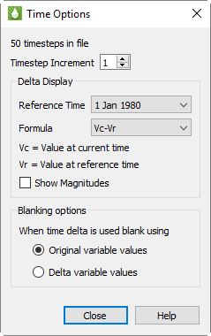
You can set the Time step Increment value to any integer between 1 and 20.
The number chosen dictates the number of time steps that each step of an
animation will advance, as well as the number of time steps that the Next
 and Previous
 buttons advance the plot. To
display the most detailed time animation (the highest number of time
steps), enter a time step increment value of "1". To view the animation,
use the Play
buttons advance the plot. To
display the most detailed time animation (the highest number of time
steps), enter a time step increment value of "1". To view the animation,
use the Play  and Rewind
 buttons in the Times region of
the sidebar.
buttons in the Times region of
the sidebar.
The Delta Display region defines the settings used to display delta values on the grid plot (by toggling-on "Time delta" in the sidebar). The delta values represent a selected relationship between the solution data at the current time step (set in the Times region of the sidebar) and the solution data at a reference time step (set in the Time Options dialog).
The reference time step, or "Ref Time", is the time step to which Tecplot RS compares each time increment in the delta value formula. Available values for the reference time step, "Ref Time", depend on your default time variable of either Time or Date (set on the Load/Save page in the Plot Options dialog). This is usually the first time step, but you can choose any time step as the reference time.
Tecplot RS supports several methods of calculating the delta value. Choosing one of the methods from the Formula menu will assign the delta calculation to use that formula.
Methods for calculating the delta value include the following, where Vc indicates the variable value at the current time and Vr indicates the variable value at the reference time:
-
Vc-Vr = Variable value at current time minus variable value at reference time (default and previously standard method)
-
Vr-Vc = Variable value at reference time minus variable value at current time
-
(Vr-Vc)/Vr = Value at reference time minus value at current time, normalized by value at reference time
-
(Vc-Vr)/Vc = Value at current time minus value at reference time, normalized by value at current time
Toggle-on "Show Magnitudes", the last option in the Delta Display region of the Time Options dialog, to use the magnitude (absolute value) of each delta value. This option ignores the direction (+ or -) of the delta value, allowing for greater display resolution.
The grid legend displays the range of variable values, as calculated based on selections in the Time Options dialog. When "Show Magnitudes" is toggled-on, a minimum range of zero displays. If you choose an unnormalized range, the legend will range from the minimum range value (either positive or negative) to the maximum value. If you choose a normalized range, the legend will vary between negative one and positive one (-1 to +1).
| You can modify the range to any positive or negative values by using the Grid Legend page of the Plot Options dialog. |
When time delta is used blank using:
When time delta is used, blanking will be applied based on either the original variable values or delta values depending on this selection. (Default: Original Values)
Settings in the Time Options dialog will display when "Time delta" is toggled-on in the sidebar.
Variable Display Controls
Depending on the plot type displayed, two or more controls appear in the sidebar next to the list of variable names. In 2D Grid plot mode, the first two controls (OWG, Delta) will display. In 3D Grid plot mode, all 8 controls display. These selections let you perform specialized computations on the variable values and show the results in the contour display.
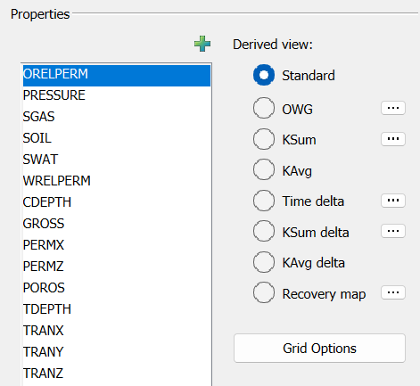
You can only use one of the options at a time. Choosing one will deselect any other. Tecplot RS may disable an option if the active grid does not have the data needed to support that function.
To learn more about the KSum, KAvg, KSum Delta, KSum Avg Delta controls, refer to KSum, KAvg, KSum/KAvg Delta Options respectively.
OWG (Oil/Water/Gas) Saturation Plots
Toggle-on "OWG" to display a ternary RGB (Red/Green/Blue) color scheme. The associated saturation variable determines the intensity of each color, where Blue = Water, Red = Gas, and Green = Oil. The legend also changes to a RGB color triangle. |
|
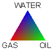
You can change the time steps or animate the plot to see how the relative oil, gas, and water saturations change over time. For example, by observing the predominantly blue regions, you can easily monitor areas with high water saturations.
Tecplot RS automatically chooses variables for Oil, Water, and Gas when possible. If your data set only includes two of these variables, Tecplot RS will automatically calculate the missing variable for you.
If the automatic choices are not suitable, you can choose the variables that represent oil, water, and gas yourself by clicking the … button next to the OWG checkbox in the sidebar. The Choose OWG Variables dialog appears.
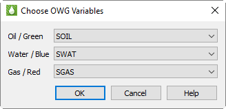
For each of oil, water, and gas, you can choose a variable using the corresponding menu. Then click OK to save your changes. The plot updates automatically after you click OK.
Time Delta
Instead of showing a variable value at a single time, you can create plots that represent the change in a variable value over time relative to a reference time step. Use the Delta toggle to do this.
When you toggle-on "Time-delta", the colors of each cell represent the variable value at the current time value in that cell, relative to a reference time step. If the slider (in the Times region of the sidebar) is at the reference (by default, the initial) time step, the entire grid will display as a solid color, representing the variable value at the minimum time value. As the time slider progresses to sequential values, the plot’s coloration will display changes in the variable value over time.
Tecplot RS will disable the Delta option when the current data set no
time-dependent variables. You can use the Delta option with the sample grid
data included in your installation (such as chelan.grid). Make
sure you have a time-dependent variable selected (with chelan.grid
loaded, chose the "PRESSURE" variable), and note the changes on your display
as you click the Play button or
other time increment buttons in the Times region of the sidebar.
Refer to Time Options for instructions on customizing the time dependency calculation settings.
Grid Options
The Grid Options dialog, accessible by clicking the Grid Options button in the Variables region of the sidebar, controls attributes of the grid display of your plot. You can use the various pages in the Grid Options dialog to customize your grid settings.
Each page of the dialog (except the Inactive Cells page) includes an Apply button. Click the Apply button to apply changes on that page of the dialog to your plot.
Orient/Thicken
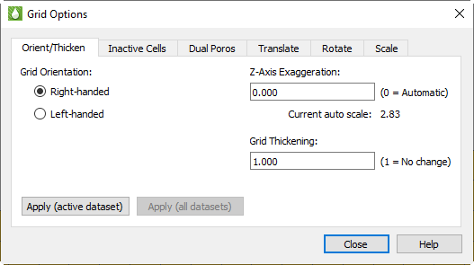
Unlike the standard topographical model where the Z-axis represents elevations (increasing upwards), reservoir simulators usually use a Depth value for the Z coordinate (that increases downward). If Tecplot RS displayed this type of grid using a typical 3D orientation, the plot would look upside-down.
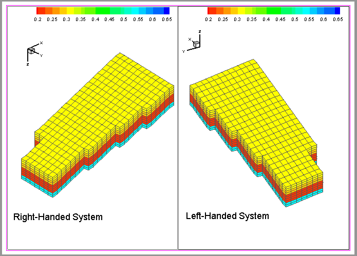
Tecplot RS provides two methods for reversing the depth component. By the first option, Tecplot RS maintains all coordinate values and rotates the 3D view so that the Z-axis points down. This maintains the right-handed nature of the coordinate system (often used by the simulator). To use this 3D view rotation, choose Right-handed as the grid orientation.
By the second method, useful for dealing with left-handed coordinate systems, Tecplot RS multiplies all Z values by -1. To use this control, choose the Left-handed grid orientation on the Orient/Thicken page of the dialog.
The two orientations result in different views of your plot; if viewed side-by-side, the same data set with the two different methods would appear as mirror images of each other
Different grid file types generally use either right or left-handed coordinate systems, and Tecplot RS chooses the most likely orientation when loading a grid file based on the file type and state file settings, in the following order.
-
Tecplot RS will use the orientation specified in the state file, if a state file exists for the file being loaded.
-
If Tecplot RS loads the file by a macro that includes orientation, it will use that setting.
-
Otherwise, Tecplot RS will choose coordinate systems based on file type:
-
Sensor grids load with right-handed coordinates,
-
VIP and VDB grids load with the coordinates specified in their files,
-
.egrid files load with left-handed coordinates unless the optional GRIDUNIT flag indicates otherwise, and
-
.grid files load with right-handed coordinates unless the optional GRIDUNIT flag indicates otherwise.
-
The Z-Axis Exaggeration value exaggerates (or flattens) the vertical scale (typically, Z). Allowable values range from 0 to 100. Use a value of 0 (recommended) to let Tecplot RS automatically compute a pleasing ratio. If you use the grid thickening factor, set the Z-Axis exaggeration to 0, at least initially.
The Grid Thickening factor allows you to stretch the Z (vertical) axis on 3D Grid plots by a selected factor, without exaggerating the topology. Especially useful for plots with thin vertical layers and irregular surfaces, this feature stretches the grid between the top and bottom surfaces, to make thin vertical layers more visible while preserving the original slopes.
While applying Z-axis scaling changes only the display, applying the Grid Thickening factor actually changes the Z values in the grid. When you apply thickening (by changing the factor to a number greater than 1), the labels on the displayed Z-axis will change, and probing results will reflect the altered Z values. Any grid equations that use the Z variable will also reflect the "stretched" Z values.
The thickening factor will default to 1 the first time a grid is loaded. Tecplot RS saves the latest factor in the project file, so that a reloaded project remembers and uses the saved factor. Multiple grids in one project may have different thickening factors.
The factor can range from 1 to 1000, where 1 indicates no thickening applied. A factor acts as a multiplier for the total grid thickness. For example, applying a thickening factor of 5 will stretch a grid with an original vertical depth of 200 to an adjusted vertical depth of 1000.
Adding a thickening factor will not thicken streamlines and survey wells (wells loaded from separate files, where those files define the well nodes with XYZ locations) with the grid. These will still display, but they may not appear at the correct depths. Wells included in the original simulation data will stretch properly with the grid.
These settings have no effect on other plot types, and you can use the thickening and exaggeration together. Click Apply (active dataset) to apply changes to the active dataset only, or Apply (all datasets) to apply changes to all currently loaded datasets.
Inactive Cells
On the Inactive Cells page of the Grid Options dialog, you can choose whether to load or unload inactive cells in the grid. You can click the Load Inactive Cells button to load the inactive cells if they are not loaded already. When Tecplot RS has inactive cells loaded, the button on this page of the dialog changes to Unload Active Cells. Click this button to immediately unload the inactive cells in your plot.
| If, when you click Load Inactive Cells, a message appears that the "Inactive grid file has not yet been solved", you must first instruct Tecplot RS to create the rsgridi file. To do this, reload your grid data, and on the Options page of the Load Grid Data dialog, either choose "Create a new RSGRID file" or toggle-on "Load inactive cells". See Loading Inactive Cells for details. |
Dual Porosity
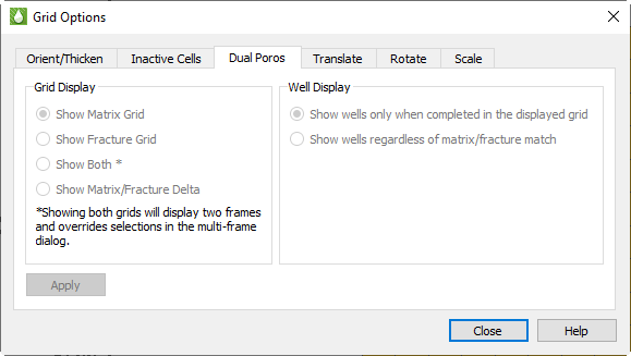
When working with dual porosity grids, you can use the Dual Poros page of the Grid Options dialog to adjust the display of matrix or fracture representations of your grid. To show both the matrix and the fracture grids simultaneously, choose "Show Both".
When displaying both grids, Tecplot RS overrides the settings in the Multi-Frame Options dialog in favor of the dual view. The two grids appear side-by-side if the paper layout is in landscape mode, or stacked vertically if the paper is in portrait mode. Refer to Paper Layout for information on changing the paper orientation.
Displaying both grids also links the view and blanking options between the two grids, regardless of the settings in the Multi-Frame Options dialog. However, layers and NNCs are still linked according to the selections in the Multi-Frame Options dialog. Cell Labels, Streams and Quick Plots appear only on the matrix grid. Finally, variable settings are linked between the frames.
For Matrix/Fracture Delta display, the left grid will show matrix cells with delta values, and the right grid will show the fracture grid. Delta is computed as follows:
-
If a cell exists in both the matrix and fracture grid, then the delta is matrix value - fracture value.
-
If a cell exists only in the matrix grid, the delta is the matrix value (matrix - 0).
-
If a cell exists only in the fracture grid, then the cell is not displayed since the delta view only shows the matrix cells.
Notes:
-
"Show Both" and "Matrix/Fracture" Delta are not available if grid "Compare" mode is enabled.
-
If the current Grid Display is "Both" or "Matrix/Fracture Delta" and the "Compare" toggle is clicked on the sidebar, the grid display will be changed to "Matrix".
-
Matrix Fracture Delta values are not displayed when viewing time step deltas.
-
Matrix/Fracture Delta values are not supported for variables created with an equation.
-
Matrix/Fracture Delta values are not exported when extracting data by cell ().
In all of the above cases, matrix values are displayed instead of the delta.
The Well Display option controls how wells are shown when displaying dual porosity grids. You may choose to display only the wells that complete in the displayed grid (first option) or to show all wells regardless of where they complete (second option). If Grid Display is set to Both, each well is shown only in the grid in which it completes (option 1), or in both grids (option 2), according to this setting.
Changing these settings requires Tecplot RS to re-output and re-draw the entire grid. Since this may take some time for large files, these settings are not applied until you explicity do so by clicking the Apply button.
Translate
You can use the Translate page of the Grid Options dialog to translate your grid to a new location relative to the coordinate system. Choose "Translate to 0,0" to shift the current minimum X and Y coordinates of the grid to the origin, or choose "Enter values" to shift the grid to a new position that you specify.
When "Enter values" is chosen as the translation, the dX, dY, and dZ text boxes become active. You can use these text boxes to indicate the direction in which you wish to shift the grid. These dX, dY, and dZ measurements reference the original grid position as dX = dY = dZ = 0. Tecplot RS reads any values in these text fields as a distance from the original position. (To undo all grid shifts, then, and return to the original grid position, type "0" into each of the three text boxes.)
With the Apply to survey wells control, you can choose whether to include survey wells in the translation. While usually survey wells require translation with the plot, turning this option off may be useful to align your plot and survey wells if the survey wells were input with a different coordinate system.
Click the Apply button to apply the translation to your plot.
Rotate
With the Rotate page of the Grid Options dialog, you can specify a rotation angle, align the edge of the grid with the axis, or use MAPAXES data if included in your data file(s).
-
Enter Angle With this control chosen, you can type the desired rotation angle (in degrees) and click Apply to rotate your plot by the specified angle.
-
Align w/ axis Choose this control to align your grid along a north/south orientation.
-
Use MAPAXES If you want to rotate an Eclipse grid, and your grid file includes MAPAXES data, you can choose this control to determine rotation (and translation if included in the MAPAXES data).
Since, as with translation, the rotation angle measures the angle from the original grid position, you can type "0" into the Rotation angle text box (and click Apply) to return the grid to its original orientation.
Toggle-on "Apply to survey wells" to rotate survey wells along with your plot, and click the Apply (active dataset) to apply changes to the active dataset only, or Apply (all datasets) to apply changes to all currently loaded datasets.
Scale
With the Scale page of the Grid Options dialog, you can multiply each coordinate by a number to scale that coordinate larger or smaller. This feature can help if you wish to convert your grid from one unit of measurement to another, or to exaggerate one dimension relative to another. (However, the Orient/Thicken controls can exaggerate the vertical dimension more optimally than the scaling controls).
Toggle-on "Apply to survey wells" to scale survey wells along with your plot.
Click the Apply (active dataset) to apply changes to the active dataset only, or Apply (all datasets) to apply changes to all currently loaded datasets.
More Grid Plot Options
Tecplot RS includes dozens of additional options for customizing the display of your grid plot. The following possibilities that you can investigate with the 3D Grid view of your plot provide an overview of your options.
On the Wells page of the Plot Options dialog, try both the Frame Units and Grid Units settings for text (click the Apply button to see the effects). Each time, zoom in and out on the grid view and watch what happens to the well labels.
On the Orient/Thicken page of the Grid Options dialog, set the Z-Axis Exaggeration Factor to "2" and click Apply. View the results, then try it again using a scale of 0 (zero).
Still on the Orient/Thicken page, set the Grid Thickening Factor to "2" and click Apply.
| See Plot Options for more information on all the features accessed with the Plot Options dialog. To learn more about grid thickening, refer to Grid Plot Axes. |
On the Grid Axes page of the Plot Options dialog, toggle-on "Show 3D Axes" and click Apply.
On the Grids page of the Plot Options dialog, switch the Contours Type to "Continuous Flood". This causes color to vary between contour levels instead of using a constant color for each cell. Look at several variables and time steps in both 2D and 3D Grid plot types, comparing them to the results you had when "Cell Center Flood" was selected.
With wells displayed, toggle-on and toggle-off "Mesh", "Contour", "Connect", "Lighting", and "Translucency" in the sidebar.
Changing Variables in Multi-frame Grid Plots
When working with multi-frame grid plots (see Using Frames), the initial multi-frame plot displays the currently chosen variable in the first frame, and subsequent variables in subsequent frames. You can change the variable chosen for each frame after the multi-frame plot has been created.
To choose a new variable for a specific frame, first make the frame active by clicking anywhere within it. Then, in the sidebar, choose the variable that you wish displayed in that frame. Tecplot RS will update that frame with new values. You can do this for each frame.