Plot Style
Scatter Plots
Scatter
- class tecplot.plot.Scatter(plot)[source]
Plot-local scatter style settings.
This class controls the style of drawn scatter points on a specific plot.
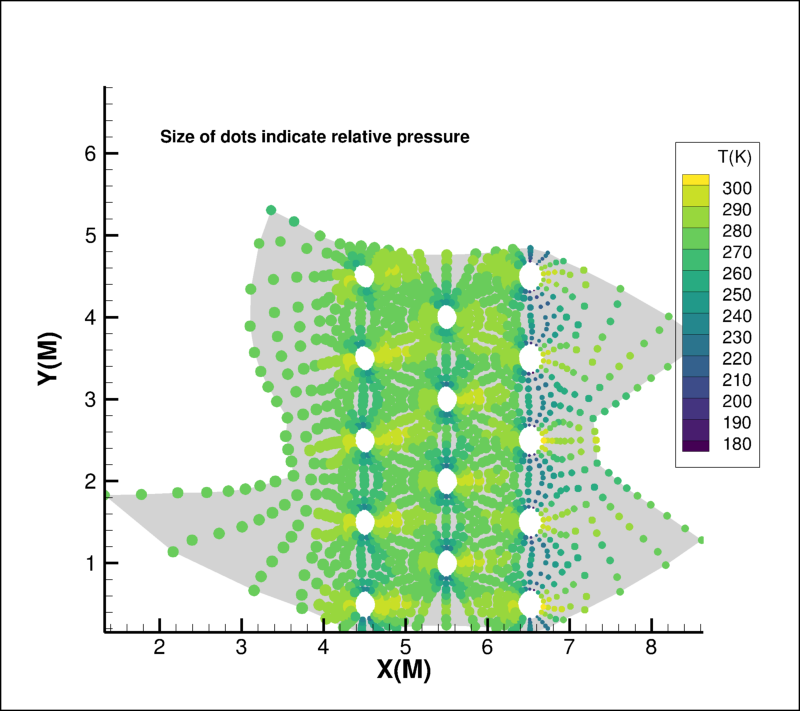
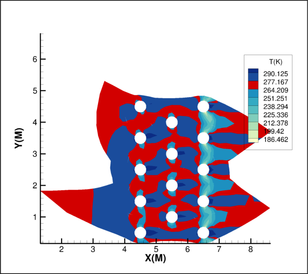
from os import path
import tecplot as tp
from tecplot.constant import *

examples_dir = tp.session.tecplot_examples_directory()
infile = path.join(examples_dir, 'SimpleData', 'HeatExchanger.plt')
dataset = tp.data.load_tecplot(infile)

frame = tp.active_frame()
frame.plot_type = PlotType.Cartesian2D
plot = frame.plot()
plot.contour(0).variable = dataset.variable('T(K)')
plot.show_scatter = True

plot.scatter.variable = dataset.variable('P(N)')

for z in dataset.zones():
    scatter = plot.fieldmap(z).scatter
    scatter.symbol_type = SymbolType.Geometry
    scatter.symbol().shape = GeomShape.Circle
    scatter.fill_mode = FillMode.UseSpecificColor
    scatter.fill_color = plot.contour(0)
    scatter.color = plot.contour(0)
    scatter.size_by_variable = True

frame.add_text('Size of dots indicate relative pressure', (20, 80))

# ensure consistent output between interactive (connected) and batch
plot.contour(0).levels.reset_to_nice()

tp.export.save_png('scatter.png')
Attributes
Default typeface to use for text scatter symbols.
Scatter symbol legend.
Reference symbol for scatter plots.
Relative size of the reference symbol.
Use grid or page units for relative size.
render quality of spheres
The
Variableto be used when sizing scatter symbols.Zero-based index of the
Variableused for size of scatter symbols.
- Scatter.base_font
Default typeface to use for text scatter symbols.
Example usage:
>>> plot.scatter.base_font.typeface = 'Times'
- Type:
- Scatter.legend
Scatter symbol legend.
Example usage:
>>> plot.scatter.legend.show = True
- Type:
- Scatter.reference_symbol
Reference symbol for scatter plots.
The reference scatter symbol is only shown when the scatter symbols are sized by a
Variablein theDataset. Example:>>> plot.fieldmap(0).scatter.size_by_variable = True >>> plot.scatter.variable = dataset.variable('s') >>> plot.scatter.reference_symbol.show = True
- Type:
- Scatter.relative_size
Relative size of the reference symbol.
Relative size will be in
cmwhen units are set toRelativeSizeUnits.Page. Example usage:>>> plot.scatter.relative_size = 20
- Type:
- Scatter.relative_size_units
Use grid or page units for relative size.
Relative size will be in
cmwhen units are set toRelativeSizeUnits.Page. Example usage:>>> from tecplot.constant import RelativeSizeUnits >>> plot.scatter.relative_size_units = RelativeSizeUnits.Grid >>> plot.scatter.relative_size = 2.0
- Type:
- Scatter.sphere_render_quality
render quality of spheres
Example usage:
>>> from tecplot.constant import * >>> plot.fieldmap(0).scatter.symbol().shape = GeomShape.Sphere >>> scatter = plot.scatter >>> scatter.sphere_render_quality = SphereScatterRenderQuality.Fast
- Scatter.variable
The
Variableto be used when sizing scatter symbols.The variable must belong to the
Datasetattached to theFramethat holds thisContourGroup. Example usage:>>> plot.scatter.variable = dataset.variable('P') >>> plot.fieldmap(0).scatter.size_by_variable = True
- Scatter.variable_index
Zero-based index of the
Variableused for size of scatter symbols.>>> plot.scatter.variable_index = dataset.variable('P').index >>> plot.fieldmap(0).scatter.size_by_variable = True
The
Datasetattached to this contour group’sFrameis used, and the variable itself can be obtained through it:>>> scatter = plot.scatter >>> scatter_var = dataset.variable(scatter.variable_index) >>> scatter_var.index == scatter.variable_index True
ScatterReferenceSymbol
- class tecplot.plot.ScatterReferenceSymbol(scatter)[source]
Reference symbol for scatter plots.
Note
The reference scatter symbol is only shown when the scatter symbols are sized by a
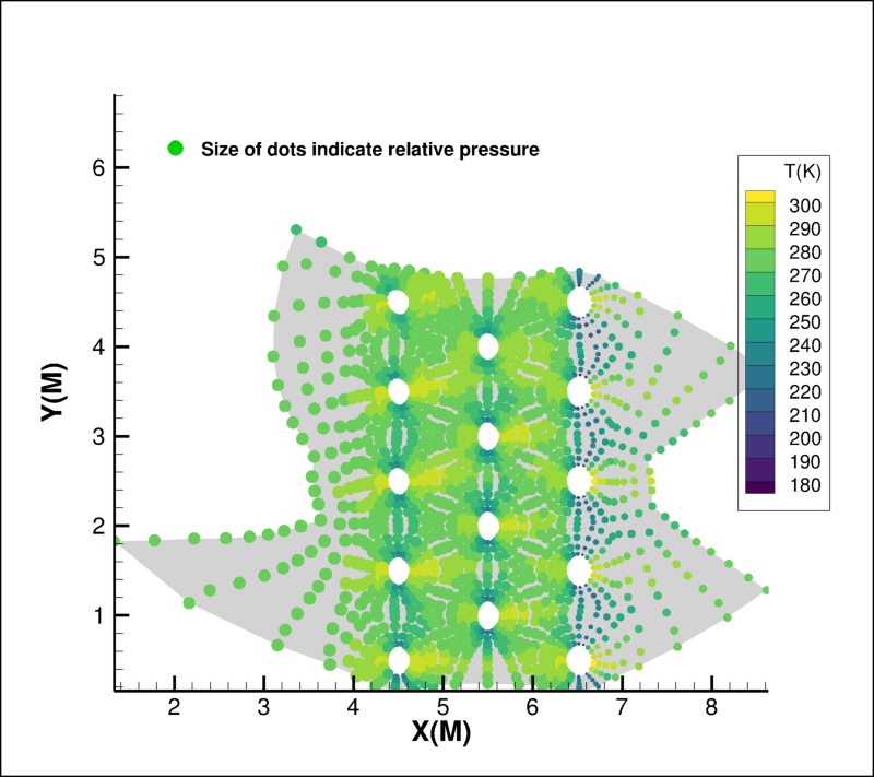
Variablein theDataset.from os import path import tecplot as tp from tecplot.constant import * examples_dir = tp.session.tecplot_examples_directory() infile = path.join(examples_dir, 'SimpleData', 'HeatExchanger.plt') dataset = tp.data.load_tecplot(infile) frame = tp.active_frame() frame.plot_type = PlotType.Cartesian2D plot = frame.plot() plot.contour(0).variable = dataset.variable('T(K)') plot.show_scatter = True plot.scatter.variable = dataset.variable('P(N)') plot.scatter.reference_symbol.show = True plot.scatter.reference_symbol.symbol().shape = GeomShape.Circle plot.scatter.reference_symbol.magnitude = plot.scatter.variable.max() plot.scatter.reference_symbol.color = Color.Green plot.scatter.reference_symbol.fill_color = Color.Green plot.scatter.reference_symbol.position = (20, 81) frame.add_text('Size of dots indicate relative pressure', (23, 80)) for z in dataset.zones(): scatter = plot.fieldmap(z).scatter scatter.symbol_type = SymbolType.Geometry scatter.symbol().shape = GeomShape.Circle scatter.fill_mode = FillMode.UseSpecificColor scatter.fill_color = plot.contour(0) scatter.color = plot.contour(0) scatter.size_by_variable = True # ensure consistent output between interactive (connected) and batch plot.contour(0).levels.reset_to_nice() tp.export.save_png('scatter_reference_symbol.png')
Attributes
The
Colorof the reference symbol.The fill
Colorof the reference symbol.Fill the background area behind the reference symbol.
Edge line thickness for geometry reference symbols.
Symbol size relative to data variable ranges.
The \((x, y)\) position of the reference symbol.
Display a reference scatter symbol on the plot.
The type of symbol to display.
Methods
symbol([symbol_type])TextSymbolorGeometrySymbol: Style control the displayed symbol.
- ScatterReferenceSymbol.color
The
Colorof the reference symbol.Example usage:
>>> from tecplot.constant import Color >>> plot.scatter.reference_symbol.color = Color.Blue
- Type:
- ScatterReferenceSymbol.fill_color
The fill
Colorof the reference symbol.Example usage:
>>> from tecplot.constant import Color >>> plot.scatter.reference_symbol.fill_color = Color.Blue
- Type:
- ScatterReferenceSymbol.filled
Fill the background area behind the reference symbol.
The background can be filled with a color or disabled (made transparent) by setting this property to
False:>>> plot.scatter.reference_symbol.filled = True
- Type:
- ScatterReferenceSymbol.line_thickness
Edge line thickness for geometry reference symbols.
Example usage:
>>> plot.scatter.reference_symbol.line_thickness = 2.5
- Type:
- ScatterReferenceSymbol.magnitude
Symbol size relative to data variable ranges.
Example usage:
>>> plot.scatter.reference_symbol.magnitude = 10.0
- Type:
- ScatterReferenceSymbol.position
The \((x, y)\) position of the reference symbol.
This position is in
Framepercentage units:>>> plot.scatter.reference_symbol.position = (50, 50)
- Type:
- ScatterReferenceSymbol.show
Display a reference scatter symbol on the plot.
Example usage:
>>> plot.fieldmap(0).scatter.size_by_variable = True
>>> plot.scatter.variable = dataset.variable('s')
>>> plot.scatter.reference_symbol.show = True
- Type:
- ScatterReferenceSymbol.symbol(symbol_type=None)[source]
TextSymbolorGeometrySymbol: Style control the displayed symbol.Example usage:
>>> from tecplot.constant import GeomShape
>>> reference_symbol = plot.scatter.reference_symbol
>>> reference_symbol.symbol = GeomShape.Sphere
- ScatterReferenceSymbol.symbol_type
The type of symbol to display.
Example usage:
>>> from tecplot.constant import SymbolType
>>> reference_symbol = plot.scatter.reference_symbol
>>> reference_symbol.symbol_type = SymbolType.Text
- Type:
Vector Plots
Vector2D
- class tecplot.plot.Vector2D(plot)[source]
Vector field style control for Cartesian 2D plots.
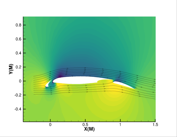
This object controls the style of the vectors that are plotted according to the vector properties under fieldmaps. The \((u,v)\) components are set using this class as well as attributes such as length, arrow-head size and the reference vector. This example shows how to show the vector field, adjusting the arrows color and thickness:
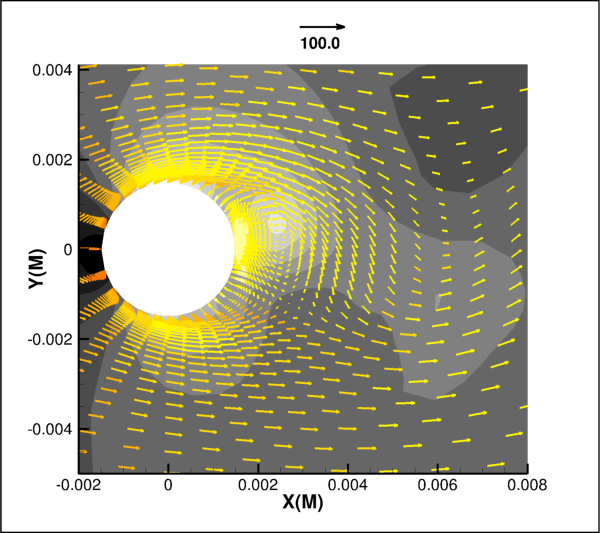
from os import path
import tecplot as tp
from tecplot.constant import *

examples_dir = tp.session.tecplot_examples_directory()
infile = path.join(examples_dir, 'SimpleData', '3ElementWing.lpk')
tp.load_layout(infile)

frame = tp.active_frame()
dataset = frame.dataset
plot = frame.plot(PlotType.Cartesian2D)

frame.background_color = Color.Black
for axis in plot.axes:
    axis.show = False

plot.axes.x_axis.min = -0.2
plot.axes.x_axis.max = 0.3
plot.axes.y_axis.min = -0.2
plot.axes.y_axis.max = 0.15

vect = plot.vector
vect.u_variable = dataset.variable('U(M/S)')
vect.v_variable = dataset.variable('V(M/S)')
vect.relative_length = 0.00025
vect.size_arrowhead_by_fraction = False
vect.arrowhead_size = 4
vect.arrowhead_angle = 10

plot.show_contour = False
plot.show_streamtraces = False
plot.show_edge = True
plot.show_vector = True

cont = plot.contour(0)
cont.variable = dataset.variable('P(N/M2)')
cont.colormap_name = 'Diverging - Blue/Yellow/Red'
cont.levels.reset_levels(80000, 90000, 100000, 110000, 120000)

plot.fieldmaps().show = False

fmap = plot.fieldmap(3)
fmap.show = True
fmap.edge.color = Color.White
fmap.edge.line_thickness = 1
fmap.points.step = 5
fmap.vector.color = cont
fmap.vector.line_thickness = 0.5

tp.export.save_png('vector2d.png', 600, supersample=3)
Attributes
Angle between the vector body and the head line.
Size of the arrowhead when sizing by fraction.
Size of arrowhead when sizing by frame height.
Spacing for even vectors.
Length of all vectors when not using relative sizing.
Vector field reference vector.
Magnitude-varying length of the vector line.
Base arrowhead size on length of vector line.
\(U\)-component
Variableof the plotted vectors.\(U\)-component
Variableindex of the plotted vectors.Use even spacing for vectors.
Use grid-units when determining the relative length.
Use relative sizing for vector lines.
\(V\)-component
Variableof the plotted vectors.\(V\)-component
Variableindex of the plotted vectors.Methods
Reset the even vector spacing.
Reset the vector length.
- Vector2D.arrowhead_angle
Angle between the vector body and the head line.
Example usage:
>>> plot.vector.arrowhead_angle = 10
- Type:
float(degrees)
- Vector2D.arrowhead_fraction
Size of the arrowhead when sizing by fraction.
The
size_arrowhead_by_fractionproperty must be set toTruefor this to take effect:>>> plot.vector.size_arrowhead_by_fraction = True >>> plot.vector.arrowhead_fraction = 0.4
- Type:
float(ratio)
- Vector2D.arrowhead_size
Size of arrowhead when sizing by frame height.
The
size_arrowhead_by_fractionproperty must be set toFalsefor this to take effect:>>> plot.vector.size_arrowhead_by_fraction = False >>> plot.vector.arrowhead_size = 4
- Type:
float(percent of frame height)
- Vector2D.even_spacing
Spacing for even vectors.
Set the spacing values in axial directions for even spaced vectors. When
use_even_spacingis turned on this will selectively remove vectors so that only one vector occupies each grid region defined by the spacing. Spacing is aligned with the X and Y axes.Example of setting spacing in X to 0.1 and Y to 0.2:
>>> plot.vector.use_even_spacing = True
>>> plot.vector.even_spacing = (0.1, 0.2)
- Type:
- Vector2D.length
Length of all vectors when not using relative sizing.
Example usage:
>>> plot.vector.use_relative = False
>>> plot.vector.length = 5
- Type:
float(percent of plot height)
- Vector2D.reference_vector
Vector field reference vector.
Example usage:
>>> plot.vector.reference_vector.show = True
- Type:
- Vector2D.relative_length
Magnitude-varying length of the vector line.
When
use_relativeisTrue, the length of the vectors will be relative to the magnitude of the velocity vector values in the data field, scaled by this parameter which is either grid-units or centimeters per unit magnitude depending on the value ofuse_grid_units:>>> plot.vector.use_relative = True >>> plot.vector.use_grid_units = True >>> plot.vector.relative_length = 0.003
- Type:
float(grid units or cm per magnitude)
- Vector2D.reset_even_spacing()
Reset the even vector spacing.
Example usage:
>>> plot.vector.reset_even_spacing()
- Vector2D.reset_length()
Reset the vector length.
Example usage:
>>> plot.vector.reset_length()
- Vector2D.size_arrowhead_by_fraction
Base arrowhead size on length of vector line.
Example usage:
>>> plot.vector.size_arrowhead_by_fraction = True
>>> plot.vector.relative_length = 0.1
- Type:
- Vector2D.u_variable
\(U\)-component
Variableof the plotted vectors.Vectors are plotted as \((u,v,w)\). Example usage:
>>> plot.vector.u_variable = dataset.variable('Pressure X')
- Type:
- Vector2D.u_variable_index
\(U\)-component
Variableindex of the plotted vectors.Vectors are plotted as \((u,v,w)\). Example usage:
>>> plot.vector.u_variable_index = 3
- Type:
int(Zero-based index)
- Vector2D.use_even_spacing
Use even spacing for vectors.
When
Truethis will selectively remove vectors from the plot to approximately enforce the display intervals specified byeven_spacing.Turn on even spacing:
>>> plot.vector.use_even_spacing = True
- Type:
- Vector2D.use_grid_units
Use grid-units when determining the relative length.
This takes effect only if
use_relativeisTrue. IfFalse,relative_lengthwill be in cm per magnitude:>>> plot.vector.use_relative = True >>> plot.vector.use_grid_units = False >>> plot.vector.relative_length = 0.010
- Type:
- Vector2D.use_relative
Use relative sizing for vector lines.
This determines whether
lengthorrelative_lengthare used to size the arrow lines. Example usage:>>> plot.vector.use_relative = False >>> plot.vector.relative_length = 0.5
- Type:
Vector3D
- class tecplot.plot.Vector3D(plot)[source]
Vector field style control for Cartesian 3D plots.
This object controls the style of the vectors that are plotted according to the vector properties under fieldmaps. The \((u,v,w)\) components are set using this class as well as attributes such as length, arrow-head size and the reference vector. See the
example for 2D vector plots.Attributes
Angle between the vector body and the head line.
Size of the arrowhead when sizing by fraction.
Size of arrowhead when sizing by frame height.
Spacing for even vectors.
Length of all vectors when not using relative sizing.
Vector field reference vector.
Magnitude-varying length of the vector line.
Base arrowhead size on length of vector line.
\(U\)-component
Variableof the plotted vectors.\(U\)-component
Variableindex of the plotted vectors.Use even spacing for vectors.
Use grid-units when determining the relative length.
Use relative sizing for vector lines.
\(V\)-component
Variableof the plotted vectors.\(V\)-component
Variableindex of the plotted vectors.\(W\)-component
Variableof the plotted vectors.\(W\)-component
Variableindex of the plotted vectors.Methods
Reset the even vector spacing.
Reset the vector length.
- Vector3D.arrowhead_angle
Angle between the vector body and the head line.
Example usage:
>>> plot.vector.arrowhead_angle = 10
- Type:
float(degrees)
- Vector3D.arrowhead_fraction
Size of the arrowhead when sizing by fraction.
The
size_arrowhead_by_fractionproperty must be set toTruefor this to take effect:>>> plot.vector.size_arrowhead_by_fraction = True >>> plot.vector.arrowhead_fraction = 0.4
- Type:
float(ratio)
- Vector3D.arrowhead_size
Size of arrowhead when sizing by frame height.
The
size_arrowhead_by_fractionproperty must be set toFalsefor this to take effect:>>> plot.vector.size_arrowhead_by_fraction = False >>> plot.vector.arrowhead_size = 4
- Type:
float(percent of frame height)
- Vector3D.even_spacing
Spacing for even vectors.
Set the spacing values in axial directions for even spaced vectors. When
use_even_spacingis turned on this will selectively remove vectors so that only one vector occupies each grid region defined by the spacing. Spacing is aligned with the X, Y, and Z axes.Example of setting spacing in X to 0.1, Y to 0.2 and Z to 0.3:
>>> plot.vector.use_even_spacing = True
>>> plot.vector.even_spacing = (0.1, 0.2, 0.3)
- Type:
- Vector3D.length
Length of all vectors when not using relative sizing.
Example usage:
>>> plot.vector.use_relative = False
>>> plot.vector.length = 5
- Type:
float(percent of plot height)
- Vector3D.reference_vector
Vector field reference vector.
Example usage:
>>> plot.vector.reference_vector.show = True
- Type:
- Vector3D.relative_length
Magnitude-varying length of the vector line.
When
use_relativeisTrue, the length of the vectors will be relative to the magnitude of the velocity vector values in the data field, scaled by this parameter which is either grid-units or centimeters per unit magnitude depending on the value ofuse_grid_units:>>> plot.vector.use_relative = True >>> plot.vector.use_grid_units = True >>> plot.vector.relative_length = 0.003
- Type:
float(grid units or cm per magnitude)
- Vector3D.reset_even_spacing()
Reset the even vector spacing.
Example usage:
>>> plot.vector.reset_even_spacing()
- Vector3D.reset_length()
Reset the vector length.
Example usage:
>>> plot.vector.reset_length()
- Vector3D.size_arrowhead_by_fraction
Base arrowhead size on length of vector line.
Example usage:
>>> plot.vector.size_arrowhead_by_fraction = True
>>> plot.vector.relative_length = 0.1
- Type:
- Vector3D.u_variable
\(U\)-component
Variableof the plotted vectors.Vectors are plotted as \((u,v,w)\). Example usage:
>>> plot.vector.u_variable = dataset.variable('Pressure X')
- Type:
- Vector3D.u_variable_index
\(U\)-component
Variableindex of the plotted vectors.Vectors are plotted as \((u,v,w)\). Example usage:
>>> plot.vector.u_variable_index = 3
- Type:
int(Zero-based index)
- Vector3D.use_even_spacing
Use even spacing for vectors.
When
Truethis will selectively remove vectors from the plot to approximately enforce the display intervals specified byeven_spacing.Turn on even spacing:
>>> plot.vector.use_even_spacing = True
- Type:
- Vector3D.use_grid_units
Use grid-units when determining the relative length.
This takes effect only if
use_relativeisTrue. IfFalse,relative_lengthwill be in cm per magnitude:>>> plot.vector.use_relative = True >>> plot.vector.use_grid_units = False >>> plot.vector.relative_length = 0.010
- Type:
- Vector3D.use_relative
Use relative sizing for vector lines.
This determines whether
lengthorrelative_lengthare used to size the arrow lines. Example usage:>>> plot.vector.use_relative = False >>> plot.vector.relative_length = 0.5
- Type:
- Vector3D.v_variable
\(V\)-component
Variableof the plotted vectors.Vectors are plotted as \((u,v,w)\). Example usage:
>>> plot.vector.v_variable = dataset.variable('Pressure Y')
- Type:
- Vector3D.v_variable_index
\(V\)-component
Variableindex of the plotted vectors.Vectors are plotted as \((u,v,w)\). Example usage:
>>> plot.vector.v_variable_index = 4
- Type:
int(Zero-based index)
ReferenceVector
- class tecplot.plot.ReferenceVector(vector)[source]
Vector field reference vector.
The reference vector is a single arrow with an optional label indicating the value of the shown reference length:
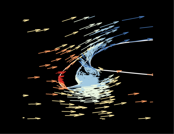
from os import path
import tecplot as tp
from tecplot.constant import *

examples_dir = tp.session.tecplot_examples_directory()
infile = path.join(examples_dir, 'SimpleData', 'VortexShedding.plt')
tp.data.load_tecplot(infile)

frame = tp.active_frame()
dataset = frame.dataset
plot = frame.plot(PlotType.Cartesian2D)

for txt in frame.texts():
    frame.delete_text(txt)

vector_contour = plot.contour(0)
vector_contour.variable = dataset.variable('T(K)')
vector_contour.colormap_name = 'Magma'
vector_contour.colormap_filter.reversed = True
vector_contour.legend.show = False
base_contour = plot.contour(1)
base_contour.variable = dataset.variable('P(N/M2)')
base_contour.colormap_name = 'GrayScale'
base_contour.colormap_filter.reversed = True
base_contour.legend.show = False

vector = plot.vector
vector.u_variable = dataset.variable('U(M/S)')
vector.v_variable = dataset.variable('V(M/S)')
vector.relative_length = 1E-5
vector.arrowhead_size = 0.2
vector.arrowhead_angle = 16

ref_vector = vector.reference_vector
ref_vector.show = True
ref_vector.position = 50, 95
ref_vector.line_thickness = 0.4
ref_vector.label.show = True
ref_vector.label.format.format_type = NumberFormat.FixedFloat
ref_vector.label.format.precision = 1
ref_vector.magnitude = 100

fmap = plot.fieldmap(0)
fmap.contour.flood_contour_group = base_contour
fmap.vector.color = vector_contour
fmap.vector.line_thickness = 0.4

plot.show_contour = True
plot.show_streamtraces = False
plot.show_vector = True

plot.axes.y_axis.min = -0.005
plot.axes.y_axis.max = 0.005
plot.axes.x_axis.min = -0.002
plot.axes.x_axis.max = 0.008

tp.export.save_png('vector2d_reference.png', 600, supersample=3)
Attributes
Degrees counter-clockwise to rotate the reference vector.
Colorof the reference vector.reference vector label style control.
reference vector line thickness.
Length of the reference vector.
\((x,y)\) of the reference vector in percent of frame height.
Draw the reference vector.
- ReferenceVector.angle
Degrees counter-clockwise to rotate the reference vector.
Example usage:
>>> ref_vector = plot.vector.reference_vector
>>> ref_vector.show = True
>>> ref_vector.angle = 90  # vertical, up
- Type:
float(degrees)
- ReferenceVector.color
Colorof the reference vector.Example usage:
>>> from tecplot.constant import Color
>>> ref_vector = plot.vector.reference_vector
>>> ref_vector.show = True
>>> ref_vector.color = Color.Red
- Type:
- ReferenceVector.label
reference vector label style control.
Example usage:
>>> ref_vector = plot.vector.reference_vector
>>> ref_vector.show = True
>>> ref_vector.label.show = True
- Type:
- ReferenceVector.line_thickness
reference vector line thickness.
Example usage:
>>> ref_vector = plot.vector.reference_vector
>>> ref_vector.show = True
>>> ref_vector.line_thickness = 0.3
- Type:
float(percentage of frame height)
- ReferenceVector.magnitude
Length of the reference vector.
Example usage:
>>> ref_vector = plot.vector.reference_vector
>>> ref_vector.show = True
>>> ref_vector.magnitude = 2
- Type:
float(data units)
- ReferenceVector.position
\((x,y)\) of the reference vector in percent of frame height.
Example usage:
>>> ref_vector = plot.vector.reference_vector
>>> ref_vector.show = True
>>> ref_vector.position = (50, 5)  # bottom, center
- Type:
ReferenceVectorLabel
- class tecplot.plot.ReferenceVectorLabel(ref_vector)[source]
Label for the reference vector.
See the example under
ReferenceVector.Attributes
Colorof the reference vector label.Typeface of the reference vector label.
Number formatting control for the reference vector label.
Distance from the reference vector to the associated label.
Print a label next to the reference vector.
- ReferenceVectorLabel.color
Colorof the reference vector label.Example usage:
>>> from tecplot.constant import Color
>>> ref_vector = plot.vector.reference_vector
>>> ref_vector.show = True
>>> ref_vector.label.show = True
>>> ref_vector.label.color = Color.Red
- Type:
- ReferenceVectorLabel.font
Typeface of the reference vector label.
Example usage:
>>> ref_vector = plot.vector.reference_vector
>>> ref_vector.show = True
>>> ref_vector.label.show = True
>>> ref_vector.label.font.size = 6
- Type:
- ReferenceVectorLabel.format
Number formatting control for the reference vector label.
Example usage:
>>> from tecplot.constant import NumberFormat
>>> ref_vector = plot.vector.reference_vector
>>> ref_vector.show = True
>>> ref_vector.label.show = True
>>> ref_vector.label.format.format_type = NumberFormat.Exponential
- Type:
Legends
ContourLegend
- class tecplot.legend.ContourLegend(contour, *svargs)[source]
Contour legend attributes.
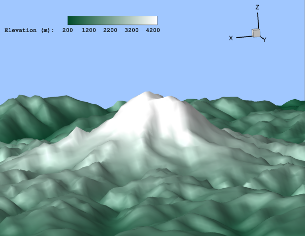
This class allows you to customize the appearance of the contour legend. The contour legend can be positioned anywhere inside the frame using the
positionattribute of this class. Example usage:import os import numpy as np import tecplot from tecplot.constant import * # By loading a layout many style and view properties are set up already examples_dir = tecplot.session.tecplot_examples_directory() datafile = os.path.join(examples_dir, 'SimpleData', 'RainierElevation.lay') tecplot.load_layout(datafile) frame = tecplot.active_frame() plot = frame.plot() # Rename the elevation variable frame.dataset.variable('E').name = "Elevation (m)" # Set the levels to nice values plot.contour(0).levels.reset_levels(np.linspace(200,4400,22)) legend = plot.contour(0).legend legend.show = True legend.vertical = False # Horizontal legend.auto_resize = False legend.label_step = 5 legend.overlay_bar_grid = False legend.position = (55, 94) # Frame percentages legend.box.box_type = TextBox.None_ # Remove Text box legend.header.font.typeface = 'Courier' legend.header.font.bold = True legend.number_font.typeface = 'Courier' legend.number_font.bold = True tecplot.export.save_png('legend_contour.png', 600, supersample=3)
Attributes
Anchor location of the legend.
Skip levels to create a reasonably sized legend.
Legend box attributes.
LegendHeaderassociated with aContourLegend.Number formatting for labels along the legend.
Spacing between labels along the contour legend.
Placement of labels on the legend.
Step size between labels along the legend.
Font used to display numbers in the legend.
Draw a line around each band in the legend color bar.
Position as a percentage of frame width/height.
Spacing between rows in the legend.
Show or hide the legend.
Show color bands for levels affected by color cutoff.
Color of legend text.
Orientation of the legend.
- ContourLegend.anchor_alignment
Anchor location of the legend.
Example usage:
>>> from tecplot.constant import PlotType, AnchorAlignment
>>> legend = frame.plot(PlotType.Cartesian3D).contour(0).legend
>>> legend.anchor_alignment = AnchorAlignment.BottomCenter
- Type:
- ContourLegend.auto_resize
Skip levels to create a reasonably sized legend.
Example usage:
>>> from tecplot.constant import PlotType
>>> legend = frame.plot(PlotType.Cartesian3D).contour(0).legend
>>> legend.auto_resize = True
- Type:
- ContourLegend.box
Legend box attributes.
Example usage:
>>> from tecplot.constant import PlotType, Color
>>> legend = frame.plot(PlotType.Cartesian3D).contour(0).legend
>>> legend.box.color = Color.Blue
- Type:
- ContourLegend.header
LegendHeaderassociated with aContourLegend.This object controls the attributes of the contour legend header.
Added in version 1.4.2: The contour legend header style control has been moved into a new namespace
header:Old API
New API
contour.legend.show_headercontour.legend.header.showcontour.legend.header_fontcontour.legend.header.fontExample usage:
>>> plot.contour(0).legend.header.show = True
- Type:
- ContourLegend.label_format
Number formatting for labels along the legend.
This is an alias for
ContourLegend.contour.labels.format:>>> contour = frame.plot().contour(0) >>> contour.legend.label_format.precision = 3 >>> print(contour.labels.format.precision) 3
- Type:
- ContourLegend.label_increment
Spacing between labels along the contour legend.
Labels will be placed on the contour variable range from min to max. The smaller the increment value the more legend labels will be created. If the
label_locationisContLegendLabelLocation.Increment, labels are incremented by this value. For example, alabel_incrementvalue of .5 will show labels at .5, 1.0, 1.5, etc.Note
This value is only used if
label_locationis set toContLegendLabelLocation.Increment. Otherwise it is ignored.Example usage:
>>> from tecplot.constant import PlotType, ContLegendLabelLocation
>>> legend = frame.plot(PlotType.Cartesian3D).contour(0).legend
>>> legend.label_location = ContLegendLabelLocation.Increment
>>> legend.label_increment = .5
See also
- Type:
- ContourLegend.label_location
Placement of labels on the legend.
If you have selected
ColorMapDistribution.Continuousfor the contour colormap filter distribution, you have three options for placement of labels on the legend:ContLegendLabelLocation.ContourLevels- This option places one label for each contour level. See Contour Levels and Color.ContLegendLabelLocation.Increment- Setlabel_incrementto the increment value.ContLegendLabelLocation.ColorMapDivisions- Places one label for each control point on the color map.
Example usage:
>>> from tecplot.constant import PlotType, ContLegendLabelLocation
>>> legend = frame.plot(PlotType.Cartesian3D).contour(0).legend
>>> legend.label_location = ContourLevelLabelLocation.Increment
>>> legend.label_increment = .5
See also
- Type:
- ContourLegend.label_step
Step size between labels along the legend.
This is an alias for
ContourLegend.contour.labels.step:>>> contour = frame.plot().contour(0) >>> contour.legend.label_step = 3 >>> print(contour.labels.step) 3
- Type:
- ContourLegend.number_font
Font used to display numbers in the legend.
Note
The font
size_unitsproperty may only be set toUnits.FrameorUnits.Point.Example usage:
>>> from tecplot.constant import PlotType
>>> legend = frame.plot(PlotType.Cartesian3D).contour(0).legend
>>> legend.number_font.italic = True
- Type:
- ContourLegend.overlay_bar_grid
Draw a line around each band in the legend color bar.
Example usage:
>>> from tecplot.constant import PlotType
>>> legend = frame.plot(PlotType.Cartesian3D).contour(0).legend
>>> legend.overlay_bar_grid = False
- Type:
- ContourLegend.position
Position as a percentage of frame width/height.
The legend is automatically placed for you. You may specify the \((x,y)\) position of the legend by setting this value, where \(x\) is the percentage of frame width, and \(y\) is a percentage of frame height.
Example usage:
>>> from tecplot.constant import PlotType
>>> legend = frame.plot(PlotType.Cartesian3D).contour(0).legend
>>> legend.position = (.1, .3)
>>> pos = legend.position
>>> pos.x  # == position[0]
.1
>>> pos.y  # == position[1]
.3
- Type:
- ContourLegend.row_spacing
Spacing between rows in the legend.
Example usage:
>>> from tecplot.constant import PlotType
>>> legend = frame.plot(PlotType.Cartesian3D).contour(0).legend
>>> legend.row_spacing = 1.5
- Type:
- ContourLegend.show
Show or hide the legend.
Example usage:
>>> from tecplot.constant import PlotType
>>> legend = frame.plot(PlotType.Cartesian3D).contour(0).legend
>>> legend.show = True
- Type:
- ContourLegend.show_cutoff_levels
Show color bands for levels affected by color cutoff.
Example usage:
>>> from tecplot.constant import PlotType
>>> legend = frame.plot(PlotType.Cartesian3D).contour(0).legend
>>> legend.show_cutoff_levels = True
- Type:
- ContourLegend.text_color
Color of legend text.
Example usage:
>>> from tecplot.constant import PlotType, Color
>>> legend = frame.plot(PlotType.Cartesian3D).contour(0).legend
>>> legend.text_color = Color.Blue
- Type:
- ContourLegend.vertical
Orientation of the legend.
When set to
True, the legend is vertical. When set toFalse, the legend is horizontal.Example usage:
>>> from tecplot.constant import PlotType
>>> legend = frame.plot(PlotType.Cartesian3D).contour(0).legend
>>> legend.vertical = False  # Show horizontal legend
- Type:
LegendHeader
- class tecplot.legend.LegendHeader(legend, *svargs)[source]
Attributes
A string to be used in the contour legend header.
Font used to display the legend header.
Show or hide the contour legend header.
Typesetter for the contour legend header.
Use custom text on the contour legend header.
- LegendHeader.custom_text
A string to be used in the contour legend header.
If the
use_custom_textproperty is set toTrue, the legend header will contain this text instead of the name of the variable assigned to the contour group. The text may contain Dynamic Text and formatting tags (see User Manual).Example usage:
>>> from tecplot.constant import PlotType
>>> plot = frame.plot(PlotType.Cartesian3D)
>>> header = plot.contour(0).legend.header
>>> header.use_custom_text = True
>>> header.custom_text = 'time: &(SOLUTIONTIME) <greek>ms</greek>'
See also:
LegendHeader.use_custom_textAdded in version 2021.2: The ability to specify custom contour legend header text requires Tecplot 360 2021 R2 or later.
Added in version 1.4.2.
- Type:
- LegendHeader.font
Font used to display the legend header.
Note
The font
size_unitsproperty may only be set toUnits.FrameorUnits.Point.Example usage:
>>> from tecplot.constant import PlotType
>>> legend = frame.plot(PlotType.Cartesian3D).contour(0).legend
>>> legend.header.font.italic = True
- Type:
- LegendHeader.show
Show or hide the contour legend header.
Note
The header text will display the name of the variable assigned to the contour group or a custom text if the
use_custom_textis set to True.Example usage:
>>> from tecplot.constant import PlotType
>>> plot = frame.plot(PlotType.Cartesian3D)
>>> legend_header = plot.contour(0).legend.header
>>> legend_header.show = True
- Type:
- LegendHeader.text_type
Typesetter for the contour legend header.
This determines how the header text for the contour legend is rendered. Options are
TextType.RegularorTextType.LaTeX. When usingLaTeX, make sure to use Python raw strings so that literal back-slashes are preserved.Example usage:
>>> from tecplot.constant import PlotType, TextType
>>> plot = frame.plot(PlotType.Cartesian3D)
>>> header = plot.contour(0).legend.header
>>> header.text_type = TextType.LaTeX
>>> header.use_custom_text = True
>>> header.custom_text = r'\LaTeX'
Added in version 2022.1: The ability to use LaTeX for contour legend header text requires Tecplot 360 2022 R1 or later.
Added in version 1.5.0.
- Type:
- LegendHeader.use_custom_text
Use custom text on the contour legend header.
If set to
True, the legend header will be set by thecustom_textproperty instead of the variable name assigned to the contour group.Example usage:
>>> from tecplot.constant import PlotType
>>> plot = frame.plot(PlotType.Cartesian3D)
>>> header = plot.contour(0).legend.header
>>> header.use_custom_text = True
>>> header.custom_text = 'Solution time: &(SOLUTIONTIME) ms'
See also:
LegendHeader.custom_textAdded in version 2021.2: The ability to specify custom contour legend header text requires Tecplot 360 2021 R2 or later.
Added in version 1.4.2.
- Type:
LineLegend
- class tecplot.legend.LineLegend(plot)[source]
Line plot legend attributes.
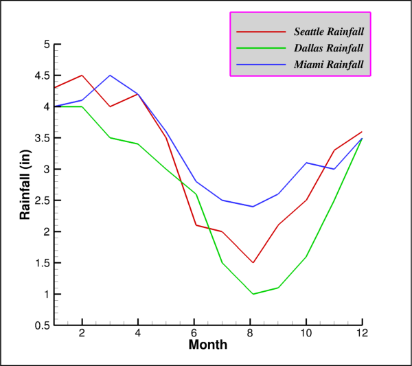
The XY line legend shows the line and symbol attributes of XY mappings. In
XY line plots, this legend includes the bar chart information. The legend can be positioned anywhere within the line plot frame by setting thepositionattribute. By default, all mappings are shown, but Tecplot 360 removes redundant entries. Example usage:import os import tecplot from tecplot.constant import * examples_dir = tecplot.session.tecplot_examples_directory() datafile = os.path.join(examples_dir, 'SimpleData', 'Rainfall.dat') dataset = tecplot.data.load_tecplot(datafile) frame = tecplot.active_frame() plot = frame.plot() frame.plot_type = tecplot.constant.PlotType.XYLine for i in range(3): plot.linemap(i).show = True plot.linemap(i).line.line_thickness = .4 y_axis = plot.axes.y_axis(0) y_axis.title.title_mode = AxisTitleMode.UseText y_axis.title.text = 'Rainfall (in)' y_axis.fit_range_to_nice() legend = plot.legend legend.show = True legend.box.box_type = TextBox.Filled legend.box.color = Color.Purple legend.box.fill_color = Color.LightGrey legend.box.line_thickness = .4 legend.box.margin = 5 legend.anchor_alignment = AnchorAlignment.MiddleRight legend.row_spacing = 1.5 legend.show_text = True legend.font.typeface = 'Arial' legend.font.italic = True legend.text_color = Color.Black legend.position = (90, 88) tecplot.export.save_png('legend_line.png', 600, supersample=3)
Attributes
Anchor location of the legend.
Legend box attributes.
Legend font attributes.
Position as a percentage of frame width/height.
Spacing between rows in the legend.
Show or hide the legend.
Show/hide mapping names in the legend.
Color of legend text.
- LineLegend.anchor_alignment
Anchor location of the legend.
Example usage:
>>> from tecplot.constant import AnchorAlignment, PlotType
>>> legend = frame.plot(PlotType.XYLine).legend
>>> legend.anchor_alignment = AnchorAlignment.BottomCenter
- Type:
- LineLegend.box
Legend box attributes.
Example usage:
>>> from tecplot.constant import PlotType, Color
>>> plot = frame.plot(PlotType.XYLine)
>>> plot.legend.box.color = Color.Blue
- Type:
- LineLegend.font
Legend font attributes.
Note
The font
size_unitsproperty may only be set toUnits.FrameorUnits.Point.Example usage:
>>> from tecplot.constant import PlotType
>>> plot = frame.plot(PlotType.XYLine)
>>> plot.legend.font.italic = True
- Type:
- LineLegend.position
Position as a percentage of frame width/height.
The legend is automatically placed for you. You may specify the \((x,y)\) position of the legend by setting this value, where \(x\) is the percentage of frame width, and \(y\) is a percentage of frame height.
Example usage:
>>> from tecplot.constant import PlotType
>>> legend = frame.plot(PlotType.XYLine).legend
>>> legend.position = (10, 30)
- Type:
- LineLegend.row_spacing
Spacing between rows in the legend.
Example usage:
>>> from tecplot.constant import PlotType
>>> legend = frame.plot(PlotType.XYLine).legend
>>> legend.row_spacing = 1.5
- Type:
- LineLegend.show
Show or hide the legend.
Example usage:
>>> from tecplot.constant import PlotType
>>> legend = frame.plot(PlotType.XYLine).legend
>>> legend.show = True
- Type:
- LineLegend.show_text
Show/hide mapping names in the legend.
Example usage:
>>> from tecplot.constant import PlotType
>>> plot = frame.plot(PlotType.XYLine)
>>> plot.legend.show_text = True
- Type:
RGBColoringLegend
- class tecplot.legend.RGBColoringLegend(rgb_coloring)[source]
Legend for RGB coloring (multivariate contour) plots.
Note
The RGB coloring legend will only show when an active fieldmap’s contour is being flooded by RGB.
import os
import numpy as np

import tecplot as tp
from tecplot.constant import *

def normalize_variable(dataset, varname, nsigma=2):
    '''
    Normalize a variable such that the specified number of standard deviations
    are within the range [0.5, 1] and the mean is transformed to 0.5. The
    new variable will append " normalized" to the original variable's name.
    '''
    with tp.session.suspend():
        newvarname = varname + ' normalized'
        dataset.add_variable(newvarname)
        data = np.concatenate([z.values(varname).as_numpy_array()
                               for z in dataset.zones()])
        vmin = data.mean() - nsigma * data.std()
        vmax = data.mean() + nsigma * data.std()
        for z in dataset.zones():
            arr = z.values(varname).as_numpy_array()
            z.values(newvarname)[:] = (arr - vmin) / (vmax - vmin)


examples_dir = tp.session.tecplot_examples_directory()
infile = os.path.join(examples_dir, 'SimpleData', 'HeatExchanger.plt')
dataset = tp.data.load_tecplot(infile)

frame = tp.active_frame()
plot = frame.plot(PlotType.Cartesian2D)
plot.show_contour = True

# Variables must be normalized relative to each other
# to make effective use of RGB coloring.
normalize_variable(dataset, 'T(K)')
normalize_variable(dataset, 'P(N)')

plot.rgb_coloring.mode = RGBMode.SpecifyGB

# all three channel variables must be set even if
# we are only contouring on two of them.
plot.rgb_coloring.red_variable = dataset.variable(0)
plot.rgb_coloring.green_variable = dataset.variable('P(N) normalized')
plot.rgb_coloring.blue_variable = dataset.variable('T(K) normalized')

plot.rgb_coloring.legend.show = True
plot.rgb_coloring.legend.green_label = 'Pressure'
plot.rgb_coloring.legend.blue_label = 'Temperature'

plot.fieldmaps().contour.flood_contour_group = plot.rgb_coloring

tp.export.save_png('rgb_coloring_legend.png')

Attributes
Anchor location of the legend.
Label to use for the blue channel.
Legend box attributes.
Legend font attributes.
Label to use for the green channel.
Size of RGB coloring legend
Placement of the RGB channels on the legend.
Position as a percentage of frame width/height.
Label to use for the red channel.
Display the RGB coloring legend.
Show the RGB channel labels.
Color of legend text.
Use the
Variablename for the blue channel.Use the
Variablename for the green channel.Use the
Variablename for the red channel.
- RGBColoringLegend.anchor_alignment
Anchor location of the legend.
Example usage:
>>> from tecplot.constant import AnchorAlignment
>>> legend = plot.rgb_coloring.legend
>>> legend.anchor_alignment = AnchorAlignment.BottomCenter
- Type:
- RGBColoringLegend.blue_label
Label to use for the blue channel.
This can be set to a string (which may be empty) but the
use_variable_for_blue_labelproperty must be set toFalsefor this label to be shown:>>> plot.rgb_coloring.legend.use_variable_for_blue_label = False >>> plot.rgb_coloring.legend.blue_label = 'water'
- Type:
- RGBColoringLegend.box
Legend box attributes.
Example usage:
>>> from tecplot.constant import Color
>>> plot.rgb_coloring.legend.box.fill_color = Color.Yellow
- Type:
- RGBColoringLegend.font
Legend font attributes.
Note
The font
size_unitsproperty may only be set toUnits.FrameorUnits.Point.Example usage:
>>> plot.rgb_coloring.legend.font.italic = True
- Type:
- RGBColoringLegend.green_label
Label to use for the green channel.
This can be set to a string (which may be empty) but the
use_variable_for_green_labelproperty must be set toFalsefor this label to be shown:>>> plot.rgb_coloring.legend.use_variable_for_green_label = False >>> plot.rgb_coloring.legend.green_label = 'oil'
- Type:
- RGBColoringLegend.height
Size of RGB coloring legend
Example usage:
>>> plot.rgb_coloring.legend.height = 20
- Type:
- RGBColoringLegend.orientation
Placement of the RGB channels on the legend.
The first color is on the bottom left, the second is on the bottom right, and the third is on top. Example usage:
>>> from tecplot.constant import RGBLegendOrientation
>>> legend = plot.rgb_coloring.legend
>>> legend.orientation = RGBLegendOrientation.RBG
- Type:
- RGBColoringLegend.position
Position as a percentage of frame width/height.
The legend is automatically placed for you. You may specify the \((x,y)\) position of the legend by setting this value, where \(x\) is the percentage of frame width, and \(y\) is a percentage of frame height.
Example usage:
>>> plot.rgb_coloring.legend.position = (20, 80)
- Type:
- RGBColoringLegend.red_label
Label to use for the red channel.
This can be set to a string (which may be empty) but the
use_variable_for_red_labelproperty must be set toFalsefor this label to be shown:>>> plot.rgb_coloring.legend.use_variable_for_red_label = False >>> plot.rgb_coloring.legend.red_label = 'gas'
- Type:
- RGBColoringLegend.show
Display the RGB coloring legend.
Example usage:
>>> plot.rgb_coloring.legend.show = True
- Type:
- RGBColoringLegend.show_labels
Show the RGB channel labels.
Example usage:
>>> legend = plot.rgb_coloring.legend
>>> legend.show_labels = True
>>> legend.red_label = 'Variable A'
>>> legend.green_label = 'Variable B'
>>> legend.blue_label = 'Variable C'
- Type:
- RGBColoringLegend.text_color
Color of legend text.
Example usage:
>>> from tecplot.constant import Color
>>> legend = plot.rgb_coloring.legend
>>> legend.text_color = Color.Blue
- Type:
- RGBColoringLegend.use_variable_for_blue_label
Use the
Variablename for the blue channel.Example usage:
>>> plot.rgb_coloring.legend.use_variable_for_blue_label = False
>>> plot.rgb_coloring.legend.blue_label = 'gas'
- Type:
ScatterLegend
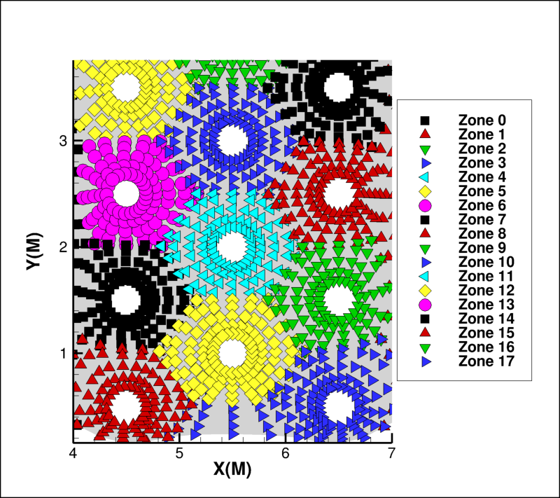
- class tecplot.legend.ScatterLegend(scatter)[source]
Legend style for scatter plots.
from os import path
import tecplot as tp
from tecplot.constant import *

examples_dir = tp.session.tecplot_examples_directory()
infile = path.join(examples_dir, 'SimpleData', 'HeatExchanger.plt')
dataset = tp.data.load_tecplot(infile)

frame = tp.active_frame()
frame.plot_type = PlotType.Cartesian2D
plot = frame.plot()
plot.show_scatter = True

# make space for the legend
plot.axes.viewport.right = 70
plot.axes.x_axis.min = 4
plot.axes.x_axis.max = 7

# assign some shape and color to each fieldmap
for i, fmap in enumerate(plot.fieldmaps()):
    for zone in fmap.zones:
        zone.name = 'Zone {}'.format(i)
    fmap.scatter.symbol().shape = GeomShape(i % 7)
    fmap.scatter.fill_mode = FillMode.UseSpecificColor
    fmap.scatter.fill_color = Color(i % 7)

plot.scatter.legend.show = True
plot.scatter.legend.row_spacing = 0.95

tp.export.save_png('scatter_legend.png')
Attributes
Anchor location of the legend.
Legend box attributes.
Legend font attributes.
Position as a percentage of frame width/height.
Spacing between rows in the legend.
Show or hide the legend.
Show/hide mapping names in the legend.
Color of legend text.
- ScatterLegend.anchor_alignment
Anchor location of the legend.
Example usage:
>>> from tecplot.constant import AnchorAlignment
>>> legend = plot.scatter.legend
>>> legend.anchor_alignment = AnchorAlignment.BottomCenter
- Type:
- ScatterLegend.box
Legend box attributes.
Example usage:
>>> from tecplot.constant import PlotType, Color
>>> plot.scatter.legend.box.color = Color.Blue
- Type:
- ScatterLegend.font
Legend font attributes.
Note
The font
size_unitsproperty may only be set toUnits.FrameorUnits.Point.Example usage:
>>> plot.scatter.legend.font.italic = True
- Type:
- ScatterLegend.position
Position as a percentage of frame width/height.
The legend is automatically placed for you. You may specify the \((x,y)\) position of the legend by setting this value, where \(x\) is the percentage of frame width, and \(y\) is a percentage of frame height.
Example usage:
>>> plot.scatter.legend.position = (10, 30)
- Type:
- ScatterLegend.row_spacing
Spacing between rows in the legend.
Example usage:
>>> plot.scatter.legend.row_spacing = 1.5
- Type:
- ScatterLegend.show
Show or hide the legend.
Example usage:
>>> plot.scatter.legend.show = True
- Type:
- ScatterLegend.show_text
Show/hide mapping names in the legend.
Example usage:
>>> plot.scatter.legend.show_text = True
- Type:
Contours
ContourGroup
- class tecplot.plot.ContourGroup(index, plot)[source]
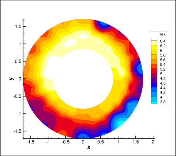
Contouring of a variable using a colormap.
This object controls the style for a specific contour group within a
Frame. Contour levels, colormap and contour lines are accessed through this class:from os import path import tecplot as tp from tecplot.constant import * # load data examples_dir = tp.session.tecplot_examples_directory() datafile = path.join(examples_dir,'SimpleData','CircularContour.plt') dataset = tp.data.load_tecplot(datafile) plot = dataset.frame.plot() plot.show_contour = True contour = plot.contour(0) contour.variable = dataset.variable('Mix') contour.colormap_name = 'Magma' # ensure consistent output between interactive (connected) and batch contour.levels.reset_to_nice() # save image to file tp.export.save_png('contour_magma.png', 600, supersample=3)
There are a fixed number of contour groups available for each plot. Others can be enabled and modified by specifying an index other than zero:
>>> contour3 = plot.contour(3)
>>> contour3.variable = dataset.variable('U')
Attributes
ContourColorCutoffobject controlling color cutoff min/max.ContourColormapFilterobject controlling colormap style properties.The name of the colormap (
str) to be used.Default target number (
int) of levels used when resetting.ContourLabelsobject controlling contour line labels.ContourLegendassociated with thisContourGroup.ContourLevelsholding the list of contour levels.ContourLinesobject controlling contour line style.The
Variablebeing contoured.Zero-based index of the
Variablebeing contoured.
- ContourGroup.color_cutoff
ContourColorCutoffobject controlling color cutoff min/max.>>> cutoff = plot.contour(0).color_cutoff >>> cutoff.min = 3.14
- Type:
- ContourGroup.colormap_filter
ContourColormapFilterobject controlling colormap style properties.>>> plot.contour(0).colormap_filter.reverse = True
- Type:
- ContourGroup.colormap_name
The name of the colormap (
str) to be used.Example:
>>> plot.contour(0).colormap_name = 'Sequential - Yellow/Green/Blue'
- Type:
- ContourGroup.default_num_levels
Default target number (
int) of levels used when resetting.Example:
>>> plot.contour(0).default_num_levels = 20
- Type:
- ContourGroup.labels
ContourLabelsobject controlling contour line labels.Lines must be turned on through the associated fieldmap object for style changes to be meaningful:
>>> plot.fieldmap(0).contour.contour_type = ContourType.Lines
>>> plot.contour(0).labels.show = True
- Type:
- ContourGroup.legend
ContourLegendassociated with thisContourGroup.This object controls the attributes of the contour legend associated with this
ContourGroup.Example usage:
>>> plot.contour(0).legend.show = True
- Type:
- ContourGroup.levels
ContourLevelsholding the list of contour levels.This object controls the values of the contour levels. Values can be added, deleted or overridden completely:
>>> plot.contour(0).levels.reset_to_nice(15)
- Type:
- ContourGroup.lines
ContourLinesobject controlling contour line style.Lines must be turned on through the associated fieldmap object for style changes to be meaningful:
>>> plot.fieldmap(0).contour.contour_type = ContourType.Lines
>>> plot.contour(0).lines.mode = ContourLineMode.DashNegative
- Type:
- ContourGroup.variable
The
Variablebeing contoured.The variable must belong to the
Datasetattached to theFramethat holds thisContourGroup. Example usage:>>> plot.contour(0).variable = dataset.variable('P')
- ContourGroup.variable_index
Zero-based index of the
Variablebeing contoured.>>> plot.contour(0).variable_index = dataset.variable('P').index
The
Datasetattached to this contour group’sFrameis used:>>> contour = plot.contour(0) >>> contour_var = frame.dataset.variable(contour.variable_index) >>> contour_var.index == contour.variable_index True
ContourColorCutoff
- class tecplot.plot.ContourColorCutoff(contour)[source]
Color-mapped value limits to display.
This lets you specify a range within which contour flooding and multi-colored objects, such as scatter symbols, are displayed:
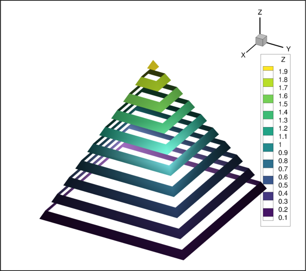
import os
import tecplot as tp
from tecplot.constant import PlotType, SurfacesToPlot

# load the data
examples_dir = tp.session.tecplot_examples_directory()
datafile = os.path.join(examples_dir,'SimpleData','Pyramid.plt')
dataset = tp.data.load_tecplot(datafile)

# show boundary faces and contours
plot = tp.active_frame().plot()
surfaces = plot.fieldmap(0).surfaces
surfaces.surfaces_to_plot = SurfacesToPlot.BoundaryFaces
plot.show_contour = True

# cutoff contour flooding outside min/max range
cutoff = plot.contour(0).color_cutoff
cutoff.include_min = True
cutoff.min = 0.5
cutoff.include_max = True
cutoff.max = 1.0
cutoff.inverted = True

# ensure consistent output between interactive (connected) and batch
plot.contour(0).levels.reset_to_nice()

tp.export.save_png('contour_color_cutoff.png',600)

Attributes
Use the maximum cutoff value.
Use the minimum cutoff value.
Cuts values outside the range instead of inside.
The maximum cutoff value.
The minimum cutoff value.
- ContourColorCutoff.include_max
Use the maximum cutoff value.
Thie example turns off the maximum cutoff:
>>> plot.contour(0).color_cutoff.include_max = False
- Type:
- ContourColorCutoff.include_min
Use the minimum cutoff value.
Example usage:
>>> plot.contour(0).color_cutoff.include_min = True
>>> plot.contour(0).color_cutoff.min = 3.14
- Type:
- ContourColorCutoff.inverted
Cuts values outside the range instead of inside.
>>> plot.contour(0).color_cutoff.inverted = True
- Type:
ContourColormapFilter
- class tecplot.plot.ContourColormapFilter(contour)[source]
Controls how the colormap is rendered for a given contour.
from os import path
import tecplot as tp
from tecplot.constant import *

# load the data
examples_dir = tp.session.tecplot_examples_directory()
datafile = path.join(examples_dir,'SimpleData','HeatExchanger.plt')
ds = tp.data.load_tecplot(datafile)

# set plot type to 2D field plot
frame = tp.active_frame()
frame.plot_type = PlotType.Cartesian2D
plot = frame.plot()

# show boundary faces and contours
surfaces = plot.fieldmap(0).surfaces
surfaces.surfaces_to_plot = SurfacesToPlot.BoundaryFaces
plot.show_contour = True

# by default, contour 0 is the one that's shown,
# set the contour's variable, colormap and number of levels
contour = plot.contour(0)
contour.variable = ds.variable('P(N)')

# cycle through the colormap three times and reversed
# show a faithful (non-approximate) continuous distribution
contour_filter = contour.colormap_filter
contour_filter.num_cycles = 3
contour_filter.reversed = True
contour_filter.fast_continuous_flood = False
contour_filter.distribution = ColorMapDistribution.Continuous

# ensure consistent output between interactive (connected) and batch
contour.levels.reset_to_nice()

# save image to file
tp.export.save_png('contour_filtered.png', 600, supersample=3)

Attributes
Upper limit for continuous colormap flooding.
Lower limit for continuous colormap flooding.
Rendering style of the colormap.
Use a fast approximation to continuously flood the colormap.
Number of cycles to repeat the colormap.
Reverse the colormap.
Enable the colormap overrides in this contour group.
Returns a
ContourColormapZebraShadefiltering object.Methods
override(index)Returns a
ContourColormapOverrideobject by index.
- ContourColormapFilter.continuous_max
Upper limit for continuous colormap flooding.
Example set the limits to the (min, max) of a variable in a specific zone:
>>> from tecplot.constant import ColorMapDistribution
>>> cmap_filter = plot.contour(0).colormap_filter
>>> cmap_filter.distribution = ColorMapDistribution.Continuous
>>> pressure = dataset.variable('Pressure').values('My Zone')
>>> cmap_filter.continuous_min = pressure.min()
>>> cmap_filter.continuous_max = pressure.max()
- Type:
- ContourColormapFilter.continuous_min
Lower limit for continuous colormap flooding.
Example usage:
>>> from tecplot.constant import ColorMapDistribution
>>> cmap_filter = plot.contour(0).colormap_filter
>>> cmap_filter.distribution = ColorMapDistribution.Continuous
>>> cmap_filter.continuous_min = 3.1415
- Type:
- ContourColormapFilter.distribution
Rendering style of the colormap.
Possible values:
BandedA solid color is assigned for all values within the band between two levels.
ContinuousThe color distribution assigns linearly varying colors to all multi-colored objects or contour flooded regions.
Example:
>>> from tecplot.constant import ColorMapDistribution
>>> cmap_filter = plot.contour(0).colormap_filter
>>> cmap_filter.distribution = ColorMapDistribution.Banded
- Type:
- ContourColormapFilter.fast_continuous_flood
Use a fast approximation to continuously flood the colormap.
Causes each cell to be flooded using interpolation between the color values at each node. When the transition from a color at one node to another node crosses over the boundary between control points in the color spectrum, fast flooding may produce colors not in the spectrum. Setting this to
Falseis slower, but more accurate:>>> cmap_filter = plot.contour(0).colormap_filter >>> cmap_filter.fast_continuous_flood = True
- Type:
- ContourColormapFilter.num_cycles
Number of cycles to repeat the colormap.
>>> plot.contour(0).colormap_filter.num_cycles = 3
- Type:
- ContourColormapFilter.override(index)[source]
Returns a
ContourColormapOverrideobject by index.- Parameters:
index (
int) – The index of the colormap override object.- Returns:
ContourColormapOverride– The class controlling the specific contour colormap override requested by index.
Example:
>>> cmap_override = plot.contour(0).colormap_filter.override(0)
>>> cmap_override.show = True
- ContourColormapFilter.reversed
Reverse the colormap.
>>> plot.contour(0).colormap_filter.reversed = True
- Type:
- ContourColormapFilter.show_overrides
Enable the colormap overrides in this contour group.
The overrides themselves must be turned on as well for this to have an effect on the resulting plot:
>>> contour = plot.contour(0)
>>> cmap_filter = contour.colormap_filter
>>> cmap_filter.show_overrides = True
>>> cmap_filter.override(0).show = True
- Type:
- ContourColormapFilter.zebra_shade
Returns a
ContourColormapZebraShadefiltering object.Example usage:
>>> zebra = plot.contour(0).colormap_filter.zebra_shade
>>> zebra.show = True
ContourColormapOverride
- class tecplot.plot.ContourColormapOverride(index, colormap_filter)[source]
Assigns contour bands to specific color.
Specific contour bands can be assigned a unique basic color. This is useful for forcing a particular region to use blue, for example, to designate an area of water. You can define up to 16 color overrides:
from os import path
import tecplot as tp
from tecplot.constant import *

# load the data
examples_dir = tp.session.tecplot_examples_directory()
datafile = path.join(examples_dir, 'SimpleData', 'HeatExchanger.plt')
dataset = tp.data.load_tecplot(datafile)

# set plot type to 2D field plot
frame = tp.active_frame()
frame.plot_type = PlotType.Cartesian2D
plot = frame.plot()

# show boundary faces and contours
surfaces = plot.fieldmap(0).surfaces
surfaces.surfaces_to_plot = SurfacesToPlot.BoundaryFaces
plot.show_contour = True

# by default, contour 0 is the one that's shown,
# set the contour's variable, colormap and number of levels
contour = plot.contour(0)
contour.variable = dataset.variable('T(K)')
contour.colormap_name = 'Sequential - Yellow/Green/Blue'
contour.levels.reset(9)

# turn on colormap overrides for this contour
contour_filter = contour.colormap_filter
contour_filter.show_overrides = True

# turn on override 0, coloring the first 4 levels red
contour_override = contour_filter.override(0)
contour_override.show = True
contour_override.color = Color.Red
contour_override.start_level = 7
contour_override.end_level = 8

# save image to file
tp.export.save_png('contour_override.png', 600, supersample=3)
Attributes
Color which will override the colormap.
Last level to override.
Include this colormap override when filter is shown.
First level to override.
- ContourColormapOverride.color
Color which will override the colormap.
Example usage:
>>> from tecplot.constant import Color
>>> colormap_filter = plot.contour(0).colormap_filter
>>> cmap_override = colormap_filter.override(0)
>>> cmap_override.color = Color.Blue
- Type:
- ContourColormapOverride.end_level
Last level to override.
Example usage:
>>> colormap_filter = plot.contour(0).colormap_filter
>>> cmap_override = colormap_filter.override(0)
>>> cmap_override.end_level = 2
- Type:
- ContourColormapOverride.show
Include this colormap override when filter is shown.
Example usage:
>>> colormap_filter = plot.contour(0).colormap_filter
>>> cmap_override = colormap_filter.override(0)
>>> cmap_override.show = True
- Type:
ContourColormapZebraShade
- class tecplot.plot.ContourColormapZebraShade(colormap_filter)[source]
This filter sets a uniform color for every other band.
Setting the color to
Noneturns the bands off and makes them transparent:from os import path import numpy as np import tecplot as tp from tecplot.constant import Color, SurfacesToPlot # load the data examples_dir = tp.session.tecplot_examples_directory() datafile = path.join(examples_dir,'SimpleData','Pyramid.plt') dataset = tp.data.load_tecplot(datafile) # show boundary faces and contours plot = tp.active_frame().plot() surfaces = plot.fieldmap(0).surfaces surfaces.surfaces_to_plot = SurfacesToPlot.BoundaryFaces plot.show_contour = True plot.show_shade = False # set zebra filter on and make the zebra contours transparent cont0 = plot.contour(0) zebra = cont0.colormap_filter.zebra_shade zebra.show = True zebra.transparent = True # ensure consistent output between interactive (connected) and batch cont0.levels.reset_to_nice() tp.export.save_png('contour_zebra.png', 600, supersample=3)
Attributes
Color of the zebra shading.
Show zebra shading in this
ContourGroup.Set the the zebra bands to be transparent.
- ContourColormapZebraShade.color
Color of the zebra shading.
Example usage:
>>> from tecplot.constant import Color
>>> filter = plot.contour(0).colormap_filter
>>> zebra = filter.zebra_shade
>>> zebra.show = True
>>> zebra.color = Color.Blue
- Type:
- ContourColormapZebraShade.show
Show zebra shading in this
ContourGroup.Example usage:
>>> cmap_filter = plot.contour(0).colormap_filter
>>> cmap_filter.zebra_shade.show = True
- Type:
ContourLabels
- class tecplot.plot.ContourLabels(contour)[source]
Contour line label style, position and alignment control.
These are labels that identify particular contour levels either by value or optionally, by number starting from one. The plot type must be lines or lines and flood in order to see them:
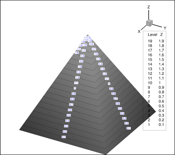
from os import path
import tecplot as tp
from tecplot.constant import Color, ContourType, SurfacesToPlot

# load the data
examples_dir = tp.session.tecplot_examples_directory()
datafile = path.join(examples_dir,'SimpleData','Pyramid.plt')
dataset = tp.data.load_tecplot(datafile)

# show boundary faces and contours
plot = tp.active_frame().plot()
plot.fieldmap(0).contour.contour_type = ContourType.Lines
surfaces = plot.fieldmap(0).surfaces
surfaces.surfaces_to_plot = SurfacesToPlot.BoundaryFaces
plot.show_contour = True

# set contour label style
contour_labels = plot.contour(0).labels
contour_labels.show = True
contour_labels.auto_align = False
contour_labels.color = Color.Blue
contour_labels.background_color = Color.White
contour_labels.margin = 20

# ensure consistent output between interactive (connected) and batch
plot.contour(0).levels.reset_to_nice()

tp.export.save_png('contour_labels.png', 600, supersample=3)
Attributes
Automatically align the labels with the contour lines.
Automatically generate labels along contour lines.
Background fill color behind the text labels.
Text color of the labels.
Fill the background area behind the text labels.
text.Fontused to show the labels.Number formatting for contour labels.
Use the contour numbers as the label instead of the data value.
Spacing around the text and the filled background area.
Show the contour line labels.
Spacing between labels along the contour lines.
Number of contour lines from one label to the next.
- ContourLabels.auto_align
Automatically align the labels with the contour lines.
This causes the flow of the text to be aligned with the contour lines. Otherwise, the labels are aligned with the frame:
>>> from tecplot.constant import ContourType
>>> plot.fieldmap(0).contour.contour_type = ContourType.Lines
>>> plot.contour(0).labels.show = True
>>> plot.contour(0).labels.auto_align = False
- Type:
- ContourLabels.auto_generate
Automatically generate labels along contour lines.
This causes a new set of contour labels to be created at each redraw:
>>> from tecplot.constant import Color, ContourType
>>> plot.fieldmap(0).contour.contour_type = ContourType.Lines
>>> plot.contour(0).labels.show = True
>>> plot.contour(0).labels.auto_generate = True
- Type:
- ContourLabels.background_color
Background fill color behind the text labels.
The
filledattribute must be set toTrue:>>> from tecplot.constant import Color, ContourType >>> plot.fieldmap(0).contour.contour_type = ContourType.Lines >>> plot.contour(0).labels.show = True >>> plot.contour(0).labels.background_color = Color.Blue
- Type:
- ContourLabels.color
Text color of the labels.
Example:
>>> from tecplot.constant import Color, ContourType
>>> plot.fieldmap(0).contour.contour_type = ContourType.Lines
>>> plot.contour(0).labels.show = True
>>> plot.contour(0).labels.color Color.Blue
- Type:
- ContourLabels.filled
Fill the background area behind the text labels.
The background can be filled with a color or disabled (made transparent) by setting this property to
False:>>> from tecplot.constant import Color, ContourType >>> plot.fieldmap(0).contour.contour_type = ContourType.Lines >>> plot.contour(0).labels.show = True >>> plot.contour(0).labels.filled = True >>> plot.contour(0).labels.background_color = Color.Blue >>> plot.contour(1).labels.show = True >>> plot.contour(1).labels.filled = False
- Type:
- ContourLabels.font
text.Fontused to show the labels.Example:
>>> from tecplot.constant import Color, ContourType
>>> plot.fieldmap(0).contour.contour_type = ContourType.Lines
>>> plot.contour(0).labels.show = True
>>> plot.contour(0).labels.font.size = 3.5
- Type:
- ContourLabels.format
Number formatting for contour labels.
Example usage:
>>> from tecplot.constant import NumberFormat
>>> contour = plot.contour(0)
>>> contour.labels.format.format_type = NumberFormat.Integer
- Type:
- ContourLabels.label_by_level
Use the contour numbers as the label instead of the data value.
Contour level numbers start from one when drawn. Example usage:
>>> from tecplot.constant import Color, ContourType
>>> plot.fieldmap(0).contour.contour_type = ContourType.Lines
>>> plot.contour(0).labels.show = True
>>> plot.contour(0).labels.label_by_level = True
- Type:
- ContourLabels.margin
Spacing around the text and the filled background area.
Contour numbers start from one when drawn. Example usage:
>>> from tecplot.constant import Color, ContourType
>>> plot.fieldmap(0).contour.contour_type = ContourType.Lines
>>> plot.contour(0).labels.show = True
>>> plot.contour(0).labels.background_color = Color.Yellow
>>> plot.contour(0).labels.margin = 20
- Type:
floatin percentage of the text height.
- ContourLabels.show
Show the contour line labels.
Contour lines must be on for this to have any effect:
>>> from tecplot.constant import ContourType
>>> plot.fieldmap(0).contour.contour_type = ContourType.Lines
>>> plot.contour(0).labels.show = True
- Type:
- ContourLabels.spacing
Spacing between labels along the contour lines.
This is the distance between each label along each contour line in percentage of the frame height:
>>> from tecplot.constant import ContourType
>>> plot.fieldmap(0).contour.contour_type = ContourType.Lines
>>> plot.contour(0).labels.show = True
>>> plot.contour(0).labels.spacing = 20
- Type:
- ContourLabels.step
Number of contour lines from one label to the next.
This is the number of contour bands between lines that are to be labeled:
>>> from tecplot.constant import ContourType
>>> plot.fieldmap(0).contour.contour_type = ContourType.Lines
>>> plot.contour(0).labels.show = True
>>> plot.contour(0).labels.step = 4
- Type:
ContourLevels
- class tecplot.plot.ContourLevels(contour)[source]
List of contour level values.
A contour level is a value at which contour lines are drawn, or for banded contour flooding, the border between different colors of flooding. Initially, each contour group consists of approximately 10 levels evenly spaced over the z coordinate in the
Frame’sDataset. These values can be manipulated with theContourLevelsobject obtained via theContourGroup.levelsattribute:from os import path import numpy as np import tecplot as tp # load layout examples_dir = tp.session.tecplot_examples_directory() example_layout = path.join(examples_dir,'SimpleData','3ElementWing.lpk') tp.load_layout(example_layout) frame = tp.active_frame() levels = frame.plot().contour(0).levels levels.reset_levels(np.linspace(55000,115000,61)) # save image to file tp.export.save_png('contour_adjusted_levels.png', 600, supersample=3)
Note
The streamtraces in the plot above is a side-effect of settings in layout file used. For more information about streamtraces, see the
plot.Streamtracesclass reference.Methods
add(*values)Adds new levels to the existing list.
delete_nearest(value)Removes the level closest to the specified value.
delete_range(min_value, max_value)Inclusively, deletes all levels within a specified range.
reset([num_levels])Resets the levels to the number specified.
reset_levels(*values)Resets the levels to the values specified.
reset_to_nice([num_levels])Approximately resets the levels to the number specified.
- ContourLevels.add(*values)[source]
Adds new levels to the existing list.
- Parameters:
*values (
floats) – The level values to be added to theContourGroup.
The values added are inserted into the list of levels in ascending order:
>>> levels = plot.contour(0).levels
>>> list(levels)
[0.0, 1.0, 2.0, 3.0, 4.0, 5.0]
>>> levels.add(3.14159)
>>> list(levels)
[0.0, 1.0, 2.0, 3.0, 3.14159, 4.0, 5.0]
- ContourLevels.delete_nearest(value)[source]
Removes the level closest to the specified value.
- Parameters:
value (
float) – Value of the level to remove.
This method deletes the contour level with the value nearest the supplied value:
>>> plot.contour(0).levels.delete_nearest(3.14)
- ContourLevels.delete_range(min_value, max_value)[source]
Inclusively, deletes all levels within a specified range.
- Parameters:
This method deletes all contour levels between the specified minimum and maximum values of the contour variable (inclusive):
>>> plot.contour(0).levels.delete_range(0.5, 1.5)
- ContourLevels.reset(num_levels=15)[source]
Resets the levels to the number specified.
- Parameters:
num_levels (
int) – Number of levels. (default: 10)
This will reset the contour levels to a set of evenly distributed values spanning the entire range of the currently selected contouring variable:
>>> plot.contour(0).levels.reset(30)
- ContourLevels.reset_levels(*values)[source]
Resets the levels to the values specified.
- Parameters:
*values (
floats) – The level values to be added to theContourGroup.
This method replaces the current set of contour levels with a new set. Here, we set the levels to go from 0 to 100 in steps of 5:
>>> plot.contour(0).levels.reset_levels(*range(0,101,5))
- ContourLevels.reset_to_nice(num_levels=15)[source]
Approximately resets the levels to the number specified.
- Parameters:
num_levels (
int) – Approximate number of levels to create. (default: 15)
This will reset the contour levels to a set of evenly distributed values that approximately spans the range of the currently selected contouring variable. Exact range and number of levels will be adjusted to make the contour levels have “nice” values:
>>> plot.contour(0).levels.reset_to_nice(50)
ContourLines
- class tecplot.plot.ContourLines(contour)[source]
Contour line style.
This object sets the style of the contour lines once turned on:
from os import path
import tecplot as tp
from tecplot.constant import (ContourLineMode, ContourType,
                              SurfacesToPlot)

# load the data
examples_dir = tp.session.tecplot_examples_directory()
datafile = path.join(examples_dir,'SimpleData','Pyramid.plt')
dataset = tp.data.load_tecplot(datafile)

# show boundary faces and contours
plot = tp.active_frame().plot()
plot.fieldmap(0).contour.contour_type = ContourType.Lines
surfaces = plot.fieldmap(0).surfaces
surfaces.surfaces_to_plot = SurfacesToPlot.BoundaryFaces
plot.show_contour = True

# set contour line style
contour_lines = plot.contour(0).lines
contour_lines.mode = ContourLineMode.SkipToSolid
contour_lines.step = 4
contour_lines.pattern_length = 2

# ensure consistent output between interactive (connected) and batch
plot.contour(0).levels.reset_to_nice()

tp.export.save_png('contour_lines.png', 600, supersample=3)

Attributes
Type of lines to draw on the plot (
ContourLineMode).Length of dashed lines and space between dashes (
float).Number of lines to step for
SkipToSolidline mode (int).
- ContourLines.mode
Type of lines to draw on the plot (
ContourLineMode).Possible values:
UseZoneLineTypeFor each zone, draw the contour lines using the line pattern and pattern length specified in the
FieldmapContourfor the parent Fieldmaps. If you are adding contour lines to polyhedral zones, the patterns will not be continuous from one cell to the next and the pattern will restart at every cell boundary.SkipToSolidDraw dashed lines between each pair of solid lines which are spaced out by the
ContourLines.stepproperty. This will override any line pattern or thickness setting in the parent Fieldmaps’sFieldmapContourobject.DashNegativeDraw lines of positive contour variable value as solid lines and lines of negative contour variable value as dashed lines. This will override any line pattern or thickness setting in the parent Fieldmaps’s
FieldmapContourobject.
Example:
>>> from tecplot.constant import ContourLineMode
>>> lines = plot.contour(0).lines
>>> lines.mode = ContourLineMode.DashNegative
- Type:
- ContourLines.pattern_length
Length of dashed lines and space between dashes (
float).The length is in percentage of the frame height:
>>> from tecplot.constant import ContourLineMode
>>> lines = plot.contour(0).lines
>>> lines.mode = ContourLineMode.SkipToSolid
>>> lines.step = 5
>>> lines.pattern_length = 5
- Type:
- ContourLines.step
Number of lines to step for
SkipToSolidline mode (int).Example:
>>> from tecplot.constant import ContourLineMode
>>> lines = plot.contour(0).lines
>>> lines.mode = ContourLineMode.SkipToSolid
>>> lines.step = 5
- Type:
RGBColoring
- class tecplot.plot.RGBColoring(plot)[source]
RGB coloring (multivariate contour) style control.
import os
import numpy as np

import tecplot as tp
from tecplot.constant import *


def normalize_variable(dataset, varname, nsigma=2):
    '''
    Normalize a variable such that the specified number of standard deviations
    are within the range [0.5, 1] and the mean is transformed to 0.5. The
    new variable will append " normalized" to the original variable's name.
    '''
    with tp.session.suspend():
        newvarname = varname + ' normalized'
        dataset.add_variable(newvarname)
        data = np.concatenate([z.values(varname).as_numpy_array()
                               for z in dataset.zones()])
        vmin = data.mean() - nsigma * data.std()
        vmax = data.mean() + nsigma * data.std()
        for z in dataset.zones():
            arr = z.values(varname).as_numpy_array()
            z.values(newvarname)[:] = (arr - vmin) / (vmax - vmin)


examples_dir = tp.session.tecplot_examples_directory()
infile = os.path.join(examples_dir, 'SimpleData', 'HeatExchanger.plt')
dataset = tp.data.load_tecplot(infile)

frame = tp.active_frame()
plot = frame.plot(PlotType.Cartesian2D)
plot.show_contour = True

# Variables must be normalized relative to each other
# to make effective use of RGB coloring.
normalize_variable(dataset, 'T(K)')
normalize_variable(dataset, 'P(N)')

plot.rgb_coloring.mode = RGBMode.SpecifyGB

# all three channel variables must be set even if
# we are only contouring on two of them.
plot.rgb_coloring.red_variable = dataset.variable(0)
plot.rgb_coloring.green_variable = dataset.variable('P(N) normalized')
plot.rgb_coloring.blue_variable = dataset.variable('T(K) normalized')

plot.rgb_coloring.legend.show = True
plot.rgb_coloring.legend.use_variable_for_green_label = False
plot.rgb_coloring.legend.green_label = 'Pressure'
plot.rgb_coloring.legend.use_variable_for_blue_label = False
plot.rgb_coloring.legend.blue_label = 'Temperature'

plot.fieldmaps().contour.flood_contour_group = plot.rgb_coloring

tp.export.save_png('rgb_coloring.png')
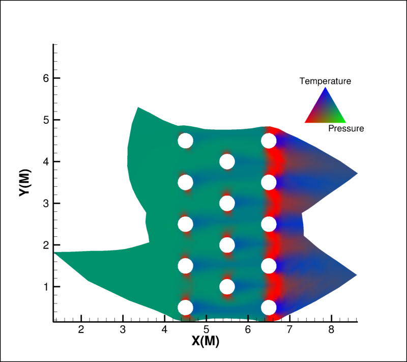
Attributes
Variableto use for the blue channel.Variableto use for the green channel.Legend placement and style control.
Variablevalue at maximum intensity for each channel.Variablevalue at minimum intensity for each channel.Which channels to use for RGB coloring.
Variableto use for the red channel.
- RGBColoring.blue_variable
Variableto use for the blue channel.Example usage:
>>> plot.rgb_coloring.blue_variable = dataset.variable('Water')
Note
In connected mode, setting this property requires Tecplot 360 version 2018 R2 or later.
- Type:
- RGBColoring.blue_variable_index
VariableIndexto use for the blue channel.Example usage:
>>> plot.rgb_coloring.blue_variable_index = 4
Note
In connected mode, setting this property requires Tecplot 360 version 2018 R2 or later.
- Type:
- RGBColoring.green_variable
Variableto use for the green channel.Example usage:
>>> plot.rgb_coloring.green_variable = dataset.variable('Oil')
Note
In connected mode, setting this property requires Tecplot 360 version 2018 R2 or later.
- Type:
- RGBColoring.green_variable_index
VariableIndexto use for the green channel.Example usage:
>>> plot.rgb_coloring.green_variable_index = 3
Note
In connected mode, setting this property requires Tecplot 360 version 2018 R2 or later.
- Type:
- RGBColoring.legend
Legend placement and style control.
Example usage:
>>> plot.rgb_coloring.legend.show = True
- Type:
- RGBColoring.max_intensity
Variablevalue at maximum intensity for each channel.This should typically be set to the maximum value of the data being plotted:
>>> plot.rgb_coloring.max_intensity = dataset.variable('P').max()
- Type:
- RGBColoring.min_intensity
Variablevalue at minimum intensity for each channel.This should typically be set to the minimum value of the data being plotted:
>>> plot.rgb_coloring.min_intensity = dataset.variable('P').min()
- Type:
- RGBColoring.mode
Which channels to use for RGB coloring.
Example usage:
>>> from tecplot.constant import RGBMode
>>> plot.rgb_coloring.mode = RGBMode.SpecifyRB
- Type:
Isosurface
IsosurfaceGroup
- class tecplot.plot.IsosurfaceGroup(index, plot)[source]
Isosurfaces style control.
import os
import tecplot as tp
from tecplot.constant import *

examples_dir = tp.session.tecplot_examples_directory()
datafile = os.path.join(examples_dir, 'OneraM6wing', 'OneraM6_SU2_RANS.plt')
dataset = tp.data.load_tecplot(datafile)

plot = tp.active_frame().plot()
plot.show_isosurfaces = True
plot.contour(0).colormap_name = 'Magma'
plot.contour(0).variable = dataset.variable('Mach')
plot.contour(0).levels.reset_levels( [.95,1.0,1.1,1.4])
plot.contour(0).legend.show = False

iso = plot.isosurface(0)
iso.show = True
iso.definition_contour_group = plot.contour(0)
iso.isosurface_selection = IsoSurfaceSelection.ThreeSpecificValues
iso.isosurface_values = [.95,1,1.1]

iso.contour.show = True
iso.contour.flood_contour_group = plot.contour(0)

iso.effects.use_translucency = True
iso.effects.surface_translucency = 80

view = plot.view
view.psi = 65.777
view.theta = 166.415
view.alpha = -1.05394
view.position = (-23.92541680486183, 101.8931504712126, 47.04269529295333)
view.width = 1.3844

tp.export.save_png('isosurface_group.png', 600, supersample=3)
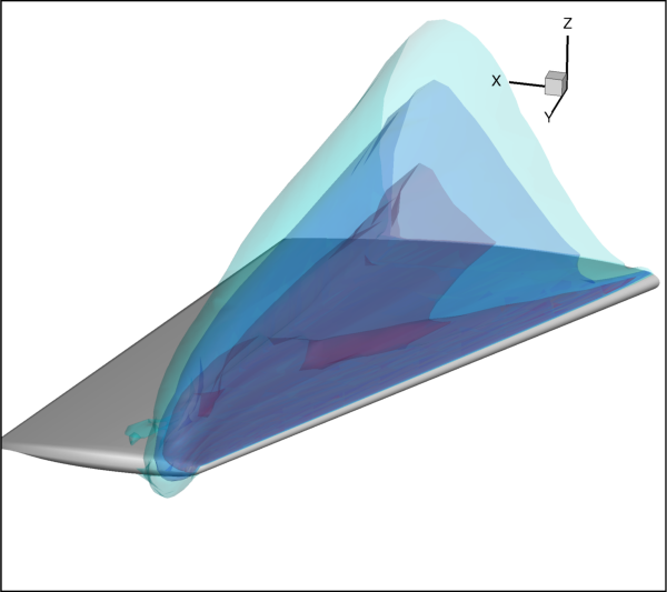
Attributes
Contour attributes for this isosurface group.
Contour group from which isosurfaces are based.
Contour group index from which isosurfaces are based.
Settings for isosurface effects.
Select where to draw isosurfaces.
Values at which to draw isosurfaces.
Mesh attributes for this isosurface group.
Obey source zone blanking.
Shade attributes for this isosurface group.
Show isosurfaces for this isosurface group.
Determines how the surface is generated.
Clip isosurface by any intersecting slices.
Vector attributes for this isosurface group.
Methods
extract([mode, assign_strand_ids])Create new zones from this isosurface.
- IsosurfaceGroup.contour
Contour attributes for this isosurface group.
Example usage:
>>> plot.isosurface(0).show = True
>>> plot.isosurface(0).contour.show = True
- Type:
- IsosurfaceGroup.definition_contour_group
Contour group from which isosurfaces are based.
Example usage:
>>> group = plot.contour(1)
>>> plot.isosurface(0).definition_contour_group = group
- Type:
- IsosurfaceGroup.definition_contour_group_index
Contour group index from which isosurfaces are based.
Contour group settings can be changed from
plot.ContourGroup.Example usage:
>>> plot.isosurface(0).show = True
>>> plot.isosurface(0).definition_contour_group_index = 1
- Type:
- IsosurfaceGroup.effects
Settings for isosurface effects.
Example usage:
>>> plot.isosurface(0).show = True
>>> plot.isosurface(0).effects.use_translucency = True
- Type:
- IsosurfaceGroup.extract(mode=ExtractMode.SingleZone, assign_strand_ids=True)[source]
Create new zones from this isosurface.
Extracts the current isosurfaces represented by this group to the
Datasetas one or more zones.- Parameters:
mode (
ExtractMode, optional) – Determines how many zones are created upon extraction. Possible values are:ExtractMode.SingleZone(default) andExtractMode.OneZonePerConnectedRegion.assign_strand_ids (
bool, optional) – Automatically assign strand ID’s to the created zones. (default:True)
- Returns:
The extracted zone if mode is
ExtractMode.SingleZone, otherwise a generator of the extracted zones.
Example usage:
>>> isosurface_zone = plot.isosurface(0).extract()
Added in version 2017.3: Isosurface extraction requires Tecplot 360 2017 R3 or later.
- IsosurfaceGroup.isosurface_selection
Select where to draw isosurfaces.
- Iso-surfaces may be drawn at:
Contour group levels
At specified value(s) - Specify up to three values of the contour variable at which to draw isosurfaces.
- To draw isosurfaces at contour group lines:
Set
isosurface_selectiontoIsoSurfaceSelection.AllContourLevels.Optional: Change
tecplot.plot.ContourLevels
- To draw isosurfaces at up to 3 values:
Set
isosurface_selectionto one of the following:IsoSurfaceSelection.OneSpecificValueIsoSurfaceSelection.TwoSpecificValuesIsoSurfaceSelection.ThreeSpecificValuesSet
isosurface_valuesto a 1, 2, or 3tupleoffloats
See also
isosurface_values.Example usage:
>>> plot.isosurface(0).show = True
>>> plot.isosurface(0).isosurface_selection = IsoSurfaceSelection.TwoSpecificValues
>>> plot.isosurface(0).isosurface_values = (.3, .8)
- Type:
- IsosurfaceGroup.isosurface_values
Values at which to draw isosurfaces.
This may be a 1, 2, or 3-
tupleoffloats, or a single scalarfloat.- To draw isosurfaces at up to 3 values:
Set
isosurface_selectionto one of the following:IsoSurfaceSelection.OneSpecificValueIsoSurfaceSelection.TwoSpecificValuesIsoSurfaceSelection.ThreeSpecificValuesSet
isosurface_valuesto a 1, 2, or 3tupleorlistoffloats, or set to a scalarfloatto assign the first value only.
When queried, this property will always return a 3 tuple of
floats.See also
isosurface_selection.Assign first isosurface value using a scalar
float:>>> plot.isosurface(0).isosurface_selection = IsoSurfaceSelection.OneSpecificValue >>> plot.isosurface(0).isosurface_values = 0.5 >>> plot.isosurface(0).isosurface_values[0] 0.5
Assign first isosurface value using a 1-
tuple:>>> plot.isosurface(0).isosurface_selection = IsoSurfaceSelection.OneSpecificValue >>> plot.isosurface(0).isosurface_values = (.5,) # 1-tuple >>> plot.isosurface(0).isosurface_values 0.5
Assign all three isosurface values:
>>> plot.isosurface(0).isosurface_selection = IsoSurfaceSelection.ThreeSpecificValues
>>> plot.isosurface(0).isosurface_values = (.5, .7, 9)
Assign the third isosurface values after assigning the first two:
>>> plot.isosurface(0).isosurface_selection = IsoSurfaceSelection.ThreeSpecificValues
>>> # Assign first and second isosurface value using a tuple
>>> plot.isosurface(0).isosurface_values = (0.0, 0.1)
>>> # Assign third isosurface value
>>> plot.isosurface(0).isosurface_values[2] = .3
>>> plot.isosurface(0).isosurface_values[2]
.3
>>> plot.isosurface(0).isosurface_values
(0.0, 0.1, .3)
Query the three isosurface values:
>>> # isosurface_values always returns a
>>> # list-like object of 3 floats with of current
>>> # isosurface values, even if fewer than three have been set.
>>> values = plot.isosurface(0).isosurface_values
>>> values
(0.1, 0.2, 0.3)
>>> values[0]
0.1
>>> values[1]
0.2
>>> values[2]
0.3
>>> len(values)
3
- IsosurfaceGroup.mesh
Mesh attributes for this isosurface group.
Example usage:
>>> plot.isosurface(0).show = True
>>> plot.isosurface(0).mesh.show = True
- Type:
- IsosurfaceGroup.obey_source_zone_blanking
Obey source zone blanking.
Example usage:
>>> plot.isosurface(0).show = True
>>> plot.isosurface(0).obey_source_zone_blanking = True
- Type:
- IsosurfaceGroup.shade
Shade attributes for this isosurface group.
Example usage:
>>> plot.isosurface(0).shade.show = True
- Type:
- IsosurfaceGroup.show
Show isosurfaces for this isosurface group.
Example usage:
>>> plot.isosurface(1).show = True
- Type:
- IsosurfaceGroup.surface_generation_method
Determines how the surface is generated.
May be one of:
SurfaceGenerationMethod.Auto:Selects one of the surface generation algorithms best suited for the zones participating in the iso-surface generation. “All polygons” is used if one or more of the participating zones is polytope, otherwise “all triangles” are used unless the iso-surface is defined by a coordinate variable in which case “allow quads” is used.
SurfaceGenerationMethod.AllPolygons:Similar to the “All triangles” method except that all interior faces generated as a result of triangulation that are not part of the original mesh are eliminated. This preserves the original mesh of the source zones on the resulting iso-surface.
SurfaceGenerationMethod.AllTriangles:An advanced algorithm that can handle complex saddle issues and guarantees that there will be no holes in the final surface. As the surface is composed entirely of triangles, it can be delivered more efficiently to the graphics hardware.
SurfaceGenerationMethod.AllowQuads:Produces quads or triangles, and the resulting surface more closely resembles the shape of the volume cells from the source zone. Since the quads are not arbitrarily divided into triangles, no biases are introduced, and the resulting surface may appear smoother. This method is preferred when the source zone is FE-Brick or IJK-Ordered and the surface is aligned with the source cells.
Example usage:
>>> from tecplot.constant import SurfaceGenerationMethod
>>> AllowQuads = SurfaceGenerationMethod.AllowQuads
>>> plot.isosurface(0).surface_generation_method = AllowQuads
- Type:
- IsosurfaceGroup.use_slice_clipping
Clip isosurface by any intersecting slices.
Example usage:
>>> from tecplot.constant import ClipPlane
>>> slice = plot.slice(0)
>>> slice.clip = ClipPlane.AbovePrimarySlice
>>> plot.fieldmap(0).effects.clip_planes = slice
>>> plot.isosurface(0).use_slice_clipping = True
See also
- Type:
- IsosurfaceGroup.vector
Vector attributes for this isosurface group.
Example usage:
>>> plot.isosurface(0).vector.show = True
- Type:
IsosurfaceContour
- class tecplot.plot.IsosurfaceContour(isosurface)[source]
Contour attributes of the isosurface group.
import os
import tecplot as tp
from tecplot.constant import *

examples_dir = tp.session.tecplot_examples_directory()
datafile = os.path.join(examples_dir, 'OneraM6wing', 'OneraM6_SU2_RANS.plt')
dataset = tp.data.load_tecplot(datafile)

plot = tp.active_frame().plot()
plot.show_isosurfaces = True
plot.contour(0).colormap_name = 'Magma'
plot.contour(0).variable = dataset.variable('Mach')
plot.contour(0).legend.show = False

iso = plot.isosurface(0)
iso.show = True
iso.definition_contour_group = plot.contour(0)
iso.isosurface_selection = IsoSurfaceSelection.OneSpecificValue
iso.isosurface_values = 1

plot.contour(1).variable = dataset.variable('Density')
iso.contour.show = True
iso.contour.contour_type = ContourType.PrimaryValue
iso.contour.flood_contour_group = plot.contour(1)

view = plot.view
view.psi = 65.777
view.theta = 166.415
view.alpha = -1.05394
view.position = (-23.92541680486183, 101.8931504712126, 47.04269529295333)
view.width = 1.3844

# ensure consistent output between interactive (connected) and batch
plot.contour(0).levels.reset_to_nice()
plot.contour(1).levels.reset_to_nice()

tp.export.save_png('isosurface_contour.png', 600, supersample=3)
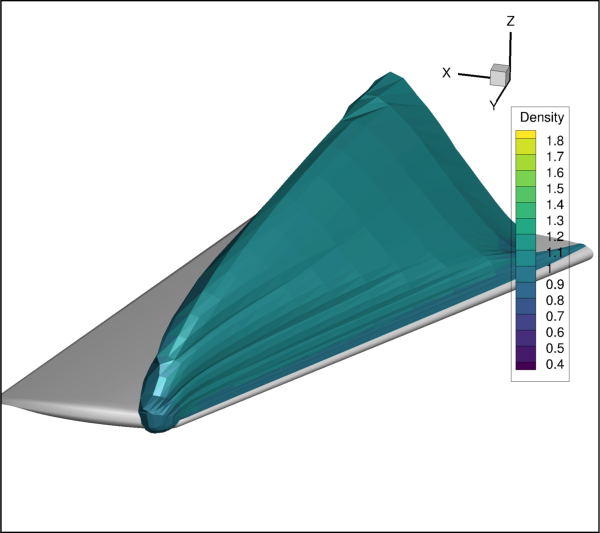
Attributes
Contour display type.
Contour group to use for flooding.
The zero-based
Indexof theContourGroupto use for flooding.Colorof contour lines.The contour group to use for contour lines.
The zero-based
Indexof theContourGroupto use for contour lines.Contour line thickness as a percentage of frame width.
Show contours on isosurfaces.
Enable lighting effect.
- IsosurfaceContour.contour_type
Contour display type.
ContourType.Lines- Draws lines of constant value of the specified contour variable.ContourType.Flood- Floods regions between contour lines with colors from a color map. The distribution of colors used for contour flooding may be banded or continuous. When banded distribution is used for flooding, a solid color is used between contour levels. If continuous color distribution is used, the flood color will vary linearly in all directions.ContourType.Overlay- Combines the above two options.ContourType.AverageCell- Floods cells or finite elements with colors from a color map according to the average value of the contour variable over the data points bounding the cell. If the variables are located at the nodes, the values at the nodes are averaged. If the variables are cell-centered, the cell-centered values are averaged to the nodes and the nodes are then averaged.ContourType.PrimaryValue- Floods cells or finite elements with colors from a color map according to the primary value of the contour variable for each cell. If the variable is cell centered, the primary value is the value assigned to the cell. If the variable is node located, the primary value comes from the lowest index node in the cell. If the variables are located at the nodes, the value of the lowest indexed node in the cell is used. When plotting IJK-ordered, FE-brick or FE-tetra cells, each face is considered independently of the other faces. You may get different colors on the different faces of the same cell. If the variables are cell-centered, the cell-centered value is used directly. When plotting I, J, or K-planes in 3D, the cell on the positive side of the plane supplies the value, except in the case of the last plane, where the cell on the negative side supplies the value.
Example usage:
>>> plot.isosurface(0).contour.show = True
>>> plot.isosurface(0).contour.contour_type = ContourType.Flood
- Type:
- IsosurfaceContour.flood_contour_group
Contour group to use for flooding.
Changing style on this
ContourGroupwill affect all fieldmaps on the sameFramethat use it.Example usage:
>>> group = plot.contour(1)
>>> contour = plot.isosurface(1).contour
>>> contour.flood_contour_group = group
- Type:
- IsosurfaceContour.flood_contour_group_index
The zero-based
Indexof theContourGroupto use for flooding.This property sets and gets, by
Index, theContourGroupused for flooding. Changing style on thisContourGroupwill affect all fieldmaps on the sameFramethat use it.Example usage:
>>> contour = plot.isosurface(0).contour
>>> contour.flood_contour_group_index = 1
- Type:
- IsosurfaceContour.line_color
Colorof contour lines.Contour lines can be a solid color or be colored by a
ContourGroupas obtained through theplot.contourproperty.Example usage:
>>> plot.show_isosurfaces = True
>>> plot.isosurface(0).contour.line_color = Color.Blue
- Type:
- IsosurfaceContour.line_contour_group
The contour group to use for contour lines.
Note that changing style on this
ContourGroupwill affect all other fieldmaps on the sameFramethat use it.Example usage:
>>> contour = plot.isosurface(0).contour
>>> group = plot.contour(1)
>>> contour.line_contour_group = group
- Type:
- IsosurfaceContour.line_contour_group_index
The zero-based
Indexof theContourGroupto use for contour lines.This property sets and gets, by
Index, theContourGroupused for line placement. Although all properties of theContourGroupcan be manipulated through this object, many of them (i.e., color) will not affect the lines unless theFieldmapContour.line_coloris set to the sameContourGroup. Note that changing style on thisContourGroupwill affect all other fieldmaps on the sameFramethat use it.Example usage:
>>> contour = plot.isosurface(0).contour
>>> contour.line_contour_group_index = 2
- Type:
- IsosurfaceContour.line_thickness
Contour line thickness as a percentage of frame width.
Suggested values are one of: .02, .1, .4, .8, 1.5
Example usage:
>>> plot.show_isosurfaces = True
>>> plot.isosurface(0).contour.line_thickness = .4
- Type:
- IsosurfaceContour.show
Show contours on isosurfaces.
Example usage:
>>> plot.isosurface(0).contour.show = True
- Type:
- IsosurfaceContour.use_lighting_effect
Enable lighting effect.
When set to
True, the lighting effect may be selected with theIsosurfaceEffects.lighting_effectattribute.Example usage:
>>> plot.isosurface(0).contour.use_lighting_effect = True
>>> plot.isosurface(0).effects.lighting_effect = LightingEffect.Paneled
- Type:
IsosurfaceEffects
- class tecplot.plot.IsosurfaceEffects(isosurface)[source]
Effects of the isosurface group.
import os
import tecplot as tp
from tecplot.constant import *

examples_dir = tp.session.tecplot_examples_directory()
datafile = os.path.join(examples_dir, 'OneraM6wing', 'OneraM6_SU2_RANS.plt')
dataset = tp.data.load_tecplot(datafile)

plot = tp.active_frame().plot()
plot.show_isosurfaces = True
plot.contour(0).colormap_name = 'Magma'
plot.contour(0).variable = dataset.variable('Mach')
plot.contour(0).legend.show = False

iso = plot.isosurface(0)
iso.show = True
iso.definition_contour_group = plot.contour(0)
iso.isosurface_selection = IsoSurfaceSelection.ThreeSpecificValues
iso.isosurface_values = [.95,1.0,1.1]

iso.effects.lighting_effect = LightingEffect.Paneled
iso.effects.use_translucency = True
iso.effects.surface_translucency = 80

view = plot.view
view.psi = 65.777
view.theta = 166.415
view.alpha = -1.05394
view.position = (-23.92541680486183, 101.8931504712126, 47.04269529295333)
view.width = 1.3844

tp.export.save_png('isosurface_effects.png', 600, supersample=3)

Attributes
Surface lighting effect.
Surface translucency of the isosurface group.
Enable surface translucency for this isosurface group.
- IsosurfaceEffects.lighting_effect
Surface lighting effect.
Isosurface lighting effects must be enabled by setting
IsosurfaceShade.use_lighting_effecttoTruewhen setting this value.There are three types of lighting effects: Paneled, SmoothWithCreases and Smooth:
Paneled: Within each cell, the color assigned to each area byshading or contour flooding is tinted by a shade constant across the cell. This shade is based on the orientation of the cell relative to your 3D light source.
SmoothUnlike
Paneledshading that colors the cell surface considering a constant angle to the light relative to the cell’s surface normal,Smoothcomputes the average normal around each cell node and interpolates the lighting influence smoothly across the cell face.SmoothWithCreasesshading is not continuous across zone boundaries unless face neighbors are specified in the data.
SmoothWithCreasesThis option is similar to
Smoothbut considers the crease angle between neighboring, connected cell faces. When the crease angle exceeds the specified amount the edge is considered creased and the lighting interpolation across the cell uses the cell’s surface normal for the shared nodes along that edge instead of the average surface normal at those nodes. If the surface has many edges that exceed the crease angle, such as a very chaotic iso-surface, a significantly larger amount of data is required to render the surface.
Example usage:
>>> plot.isosurface(0).shade.use_lighting_effect = True
>>> plot.isosurface(0).effects.lighting_effect = LightingEffect.Paneled
- Type:
- IsosurfaceEffects.surface_translucency
Surface translucency of the isosurface group.
Iso-surface surface translucency must be enabled by setting
IsosurfaceEffects.use_translucency=Truewhen setting this value.Valid translucency values range from one (opaque) to 99 (translucent).
Example usage:
>>> plot.isosurface(0).effects.use_translucency = True
>>> plot.isosurface(0).effects.surface_translucency = 20
- Type:
- IsosurfaceEffects.use_translucency
Enable surface translucency for this isosurface group.
The surface translucency value can be changed by setting
IsosurfaceEffects.surface_translucency.Example usage:
>>> plot.isosurface(0).effects.use_translucency = True
>>> plot.isosurface(0).effects.surface_translucency = 20
- Type:
IsosurfaceMesh
- class tecplot.plot.IsosurfaceMesh(isosurface)[source]
Mesh attributes of the isosurface group.
import os
import tecplot as tp
from tecplot.constant import *

examples_dir = tp.session.tecplot_examples_directory()
datafile = os.path.join(examples_dir, 'OneraM6wing', 'OneraM6_SU2_RANS.plt')
dataset = tp.data.load_tecplot(datafile)

plot = tp.active_frame().plot()
plot.show_isosurfaces = True
plot.contour(0).colormap_name = 'Magma'
plot.contour(0).variable = dataset.variable('Mach')
plot.contour(0).legend.show = False

iso = plot.isosurface(0)
iso.show = True
iso.definition_contour_group = plot.contour(0)
iso.isosurface_selection = IsoSurfaceSelection.OneSpecificValue
iso.isosurface_values = 1
iso.mesh.show = True
iso.mesh.color = Color.Mahogany
iso.mesh.line_thickness = 0.4

view = plot.view
view.psi = 65.777
view.theta = 166.415
view.alpha = -1.05394
view.position = (-23.92541680486183, 101.8931504712126, 47.04269529295333)
view.width = 1.3844

tp.export.save_png('isosurface_mesh.png', 600, supersample=3)
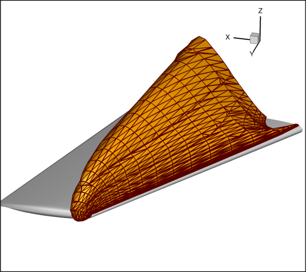
Attributes
Isosurface mesh color.
Isosurface mesh line thickness.
Display the mesh on isosurfaces.
- IsosurfaceMesh.color
Isosurface mesh color.
Iso-surface mesh lines can be a solid color or be colored by a
ContourGroupas obtained through theplot.contourproperty.Example usage:
>>> plot.isosurface(0).mesh.show = True
>>> plot.isosurface(0).mesh.color = Color.Blue
- Type:
- IsosurfaceMesh.line_thickness
Isosurface mesh line thickness.
Suggested values are .002, .1, .4, .8, 1.5
Example usage:
>>> plot.isosurface(0).mesh.show = True
>>> plot.isosurface(0).mesh.line_thickness = .4
- Type:
IsosurfaceShade
- class tecplot.plot.IsosurfaceShade(isosurface)[source]
Shade attributes of the isosurface group.
import tecplot as tp
from os import path
from tecplot.plot import IsosurfaceGroup
from tecplot.constant import Color, LightingEffect

examples_dir = tp.session.tecplot_examples_directory()
datafile = path.join(examples_dir, 'SimpleData', 'DuctFlow.plt')
dataset = tp.data.load_tecplot(datafile)

plot = tp.active_frame().plot()
plot.show_isosurfaces = True
plot.contour(0).variable = dataset.variable('U(M/S)')
iso = plot.isosurface(0)

iso.contour.show = False  # Hiding the contour will reveal the shade.

iso.shade.show = True
iso.shade.color = Color.Red
iso.shade.use_lighting_effect = True

iso.effects.lighting_effect = LightingEffect.Paneled

tp.export.save_png('isosurface_shade.png', 600, supersample=3)
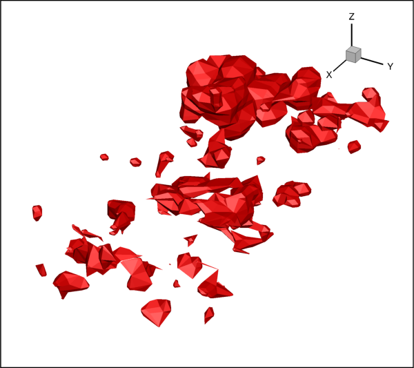
Attributes
Shade color.
Show shade attributes.
Enable lighting effect.
- IsosurfaceShade.color
Shade color.
Color.MultiColorandColor.RGBColorcoloring are not available. Use flooded contours for multi-color or RGB floodingExample usage:
>>> plot.isosurface(0).shade.show = True
>>> plot.isosurface(0).shade.color = Color.Blue
- Type:
- IsosurfaceShade.show
Show shade attributes.
Example usage:
>>> plot.isosurface(0).shade.show = True
- Type:
- IsosurfaceShade.use_lighting_effect
Enable lighting effect.
When set to
True, the lighting effect may be selected with theIsosurfaceEffects.lighting_effectattribute.Example usage:
>>> plot.isosurface(0).shade.use_lighting_effect = True
>>> plot.isosurface(0).effects.lighting_effect = LightingEffect.Paneled
- Type:
IsosurfaceVector
- class tecplot.plot.IsosurfaceVector(isosurface)[source]
Isosurface vector field control.
Added in version 2017.3: Isosurface vectors requires Tecplot 360 2017 R3 or later.
import os
import tecplot as tp
from tecplot.constant import *

examples_dir = tp.session.tecplot_examples_directory()
datafile = os.path.join(examples_dir, 'SimpleData', 'DuctFlow.plt')
dataset = tp.data.load_tecplot(datafile)

plot = tp.active_frame().plot()
plot.contour(0).variable = dataset.variable('T(K)')
plot.contour(1).variable = dataset.variable('P(N/m2)')
plot.vector.u_variable = dataset.variable('U(M/S)')
plot.vector.v_variable = dataset.variable('V(M/S)')
plot.vector.w_variable = dataset.variable('W(M/S)')

plot.show_isosurfaces = True
plot.contour(0).legend.show = False
plot.contour(1).legend.show = False

iso = plot.isosurface(0)
iso.definition_contour_group = plot.contour(0)
iso.contour.flood_contour_group = plot.contour(1)
iso.isosurface_values = 200
iso.show = True

iso.vector.show = True
iso.vector.line_thickness = 0.4
iso.vector.color = Color.Grey

view = plot.view
view.psi = 53.80
view.theta = -139.15
view.alpha = 0
view.position = (7.54498, 8.42026, 7.94559)
view.width = 0.551882

tp.export.save_png('isosurface_vector.png', 600, supersample=3)

Attributes
Arrowhead style of isosurface vectors.
Isosurface vector color.
Use tangent vectors for isosurfaces.
Vector line thickness as a percentage of the frame height.
Show vectors on isosurfaces.
Type of vector for isosurfaces.
- IsosurfaceVector.arrowhead_style
Arrowhead style of isosurface vectors.
Example usage:
>>> isosurface_vector = plot.isosurface(0).vector
>>> isosurface_vector.show = True
>>> isosurface_vector.arrowhead_style = ArrowheadStyle.Hollow
Added in version 2017.3: Isosurface vectors requires Tecplot 360 2017 R3 or later.
- Type:
- IsosurfaceVector.color
Isosurface vector color.
Iso-surface vectors can be a solid color or be colored by a
ContourGroupas obtained through theplot.contourproperty.Example usage:
>>> plot.isosurface(0).vector.show = True
>>> plot.isosurface(0).vector.color = Color.Blue
Added in version 2017.3: Isosurface vectors requires Tecplot 360 2017 R3 or later.
- Type:
- IsosurfaceVector.is_tangent
Use tangent vectors for isosurfaces.
Example usage:
>>> plot.isosurface(0).vector.show = True
>>> plot.isosurface(0).vector.is_tangent = True
Added in version 2017.3: Isosurface vectors requires Tecplot 360 2017 R3 or later.
- Type:
- IsosurfaceVector.line_thickness
Vector line thickness as a percentage of the frame height.
Typical values are .02, .1, .4, .8, 1.5
Example usage:
>>> plot.isosurface(0).vector.show = True
>>> plot.isosurface(0).vector.line_thickness = .1
Added in version 2017.3: Isosurface vectors requires Tecplot 360 2017 R3 or later.
- Type:
- IsosurfaceVector.show
Show vectors on isosurfaces.
Example usage:
>>> plot.isosurface(0).vector.show = True
Added in version 2017.3: Isosurface vectors requires Tecplot 360 2017 R3 or later.
- Type:
- IsosurfaceVector.vector_type
Type of vector for isosurfaces.
Example usage:
>>> plot.isosurface(0).vector.show = True
>>> plot.isosurface(0).vector.vector_type = VectorType.MidAtPoint
Added in version 2017.3: Isosurface vectors requires Tecplot 360 2017 R3 or later.
- Type:
Slice
SliceGroup
- class tecplot.plot.SliceGroup(plot, index)[source]
Change attributes associated with a specific slice group.
Slices can include lighting effects, contours, meshes, and more. To customize these and other attributes of slices, use this object.
This object controls the style for a specific slice group within a
Frame. Slicecontour, vector, edge, effects, mesh, visibility and position information are accessed through this class:from os import path import tecplot as tp from tecplot.constant import * examples_dir = tp.session.tecplot_examples_directory() datafile = path.join(examples_dir, 'SimpleData', 'DuctFlow.plt') dataset = tp.data.load_tecplot(datafile) plot = tp.active_frame().plot() plot.contour(0).variable = dataset.variable('U(M/S)') plot.show_edge = True plot.fieldmap(0).edge.edge_type = EdgeType.Creases vectors = plot.vector vectors.u_variable = dataset.variable('U(M/S)') vectors.v_variable = dataset.variable('V(M/S)') vectors.w_variable = dataset.variable('W(M/S)') plot.show_slices = True slice_0 = plot.slice(0) slice_0.contour.show = True slice_0.contour.contour_type = ContourType.Overlay # AKA "Both lines and flood" slice_0.effects.use_translucency = True slice_0.effects.surface_translucency = 30 # Show an arbitrary slice slice_0.orientation = SliceSurface.Arbitrary slice_0.arbitrary_normal = (1, .5, 0) slice_0.show_primary_slice = False slice_0.show_start_and_end_slices = True slice_0.start_position = (-.21, .05, .025) slice_0.end_position = (1.342, .95, .475) slice_0.show_intermediate_slices = True slice_0.num_intermediate_slices = 3 slice_0.edge.show = True slice_0.edge.line_thickness = 0.4 # ensure consistent output between interactive (connected) and batch plot.contour(0).levels.reset_to_nice() tp.export.save_png('slice_group.png', 600, supersample=3)
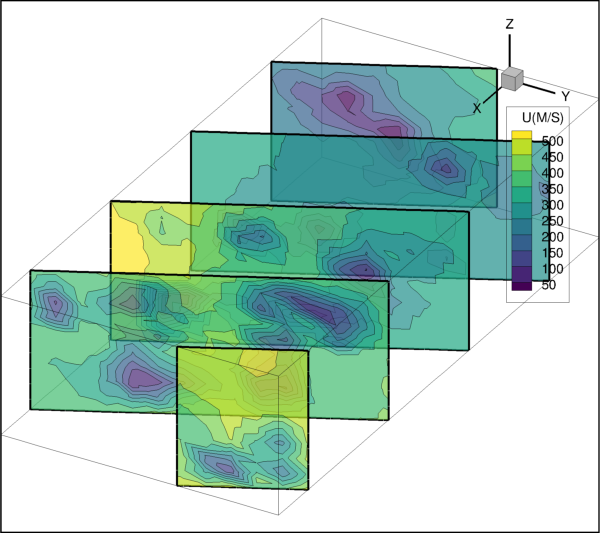
Up to eight different slice groups can be set. Each slice group can use different slice planes or different ranges for the same slice plane.
>>> slice_3 = plot.slice(3)
>>> slice_3.contour.show = True
See also
Attributes
Normal for arbitrary slices.
Orientation of data clipping for this slice group.
Contour attributes for the slice group.
Edge attributes for this slice group.
Effects attributes for this slice group.
Position of the end slice.
Mesh attributes for this slice group.
Number of intermediate slicing planes.
Obey source zone blanking.
Select on which plane the slice is drawn.
Origin of the slice.
Shade attributes for this slice group.
Show slices for this slice group.
Show intermediate slices.
bool; Include the primary slice (first slice placed) in the Plot.Include start and end slices.
SliceSource: Zones to slice through.Position of the start slice.
Determines how the surface is generated.
Clip this slice by any intersecting slices.
Vector attributes for this slice group.
Methods
extract([mode, assign_strand_ids, ...])Create new zones from this slice.
set_arbitrary_from_points(p1, p2, p3)Set an arbitrary slice from 3 points.
- SliceGroup.arbitrary_normal
Normal for arbitrary slices.
Example usage:
>>> plot.slice(0).orientation = SliceSurface.Arbitrary
>>> plot.slice(0).arbitrary_normal = (0.1, 0.2, 0.3)
>>> plot.slice(0).arbitrary_normal.x
0.1
>>> plot.slice(0).arbitrary_normal.y
0.2
>>> plot.slice(0).arbitrary_normal.z
0.3
- Type:
- SliceGroup.clip
Orientation of data clipping for this slice group.
Clipping the field data, isosurfaces, streamtraces or other plot objects using slices requires setting the
clipproperty of the slice as well as adding the slice group to theclip_planesproperty on the fieldmap effects. Only slice groups 0 to 5 are available for clipping in this framework:>>> from tecplot.constant import * >>> # setup slice and clipping orientation >>> slice = plot.slice(0) >>> slice.origin = (7, 0, 0) >>> slice.clip = ClipPlane.AbovePrimarySlice >>> # add slice group to the fieldmap clip planes >>> plot.fieldmap(0).effects.clip_planes = [slice] >>> # turn on and set value of isosurface >>> # and enforce slice clipping >>> isosurf = plot.isosurface(0) >>> isosurf.isosurface_values = 3 >>> isosurf.use_slice_clipping = True >>> # turn on isosurfaces and slices >>> pt.show_isosurfaces = True >>> pt.show_slices = True
Warning
Slice clipping is only supported for X, Y and Z-planes.
Slice clipping has no effect for slices that have an orientation of
SliceSurface.Arbitrary,SliceSurface.IPlanes,SliceSurface.JPlanesor ,SliceSurface.KPlanes. That is, the orientation must be one of:SliceSurface.XPlanes,SliceSurface.YPlanesorSliceSurface.ZPlanes.- Type:
- SliceGroup.contour
Contour attributes for the slice group.
Example usage:
>>> plot.slice(0).contour.show = True
- Type:
- SliceGroup.edge
Edge attributes for this slice group.
Example usage:
>>> plot.slice(0).edge.show = True
- Type:
- SliceGroup.effects
Effects attributes for this slice group.
Example usage:
>>> plot.slice(0).effects.use_translucency = True
- Type:
- SliceGroup.end_position
Position of the end slice.
SliceGroup.show_start_and_end_slicesmust beTrueto show the end slice. This will be a 3-tupleoffloatiforientationisX,Y,Zor zero-basedintiforientationisI,J,K.Example usage:
>>> plot.slice(0).show_start_and_end_slices = True
>>> plot.slice(0).end_position = (1, 1, 1)
>>> plot.slice(0).end_position.i
1
- SliceGroup.extract(mode=ExtractMode.SingleZone, assign_strand_ids=True, resulting_1d_zone_type=Resulting1DZoneType.IOrderedIfPossible, transient_mode=TransientOperationMode.SingleSolutionTime)[source]
Create new zones from this slice.
Extracts the current slices represented by this group to the
Datasetas one or more zones.- Parameters:
mode (
ExtractMode, optional) – Determines how many zones are created upon extraction. Possible values are:ExtractMode.SingleZone(default) andExtractMode.OneZonePerConnectedRegion.assign_strand_ids (
bool, optional) – Automatically assign strand ID’s to the created zones. (default:True)resulting_1d_zone_type (
Resulting1DZoneType, optional) – The type of zone to create when the result is one-dimensional. Possible values are:Resulting1DZoneType.IOrderedIfPossible(default) andResulting1DZoneType.FELineSegment.transient_mode (
TransientOperationMode) – Determines which solution times are used to extract slices when transient data is available in the dataset. Possible values areTransientOperationMode.SingleSolutionTime(default) orTransientOperationMode.AllSolutionTimes.
- Returns:
The extracted zone is returned if mode is
ExtractMode.SingleZoneand transient_mode isTransientOperationMode.SingleSolutionTime, otherwise a generator of the extracted zones.
See also
Example usage:
>>> slice_zone = plot.slice(0).extract()
- SliceGroup.indices
- SliceGroup.mesh
Mesh attributes for this slice group.
Example usage:
>>> plot.slice(0).mesh.show = True
- Type:
- SliceGroup.num_intermediate_slices
Number of intermediate slicing planes.
You may specify between 1 and 5,000 intermediate slices.
Example usage:
>>> # Show 2 intermediate slices
>>> plot.slice(0).num_intermediate_slices = 2
- Type:
- SliceGroup.obey_source_zone_blanking
Obey source zone blanking.
When set to
True, slices are subject to any blanking used for the data. When set toFalse, slices are generated for blanked and unblanked regions.Example usage:
>>> plot.slice(0).obey_source_zone_blanking = True
- Type:
- SliceGroup.orientation
Select on which plane the slice is drawn.
You may also choose
SliceSurface.Arbitraryto place the slice on an arbitrary plane.To orient slices in an arbitrary direction, choose
SliceSurface.Arbitrary. As with other slices, you may specify origin points for a primary slice and/or for start and end slices. Slices pass through the indicated origin point(s), so you can easily align the edge of a slice or group of slices along some other feature of the plot, such as an axis. If intermediate slices are activated, they are drawn equally spaced between the slices defined by the start and end origins.Example usage:
>>> plot.slice(0).orientation = SliceSurface.XPlanes
- Type:
- SliceGroup.origin
Origin of the slice.
This will be a 3-
tupleoffloatiforientationisX,Y,Zor zero-basedintiforientationisI,J,K. For arbitrary slice orientation, the origin can be any location. For axis orientations (XPlanes,YPlanes, etc.) two of the three components are not used.Example usage:
>>> slice_0 = plot.slice(0)
>>> slice_0.orientation = SliceSurface.IPlanes
>>> slice_0.origin = (1, 0, 0)
>>> dx = (1, 1, 1)
>>> slice_0.origin += dx
>>> slice_0.origin.i
2
>>> slice_0.origin.j
1
>>> slice_0.origin.k
1

>>> slice_0.orientation = SliceSurface.Arbitrary
>>> slice_0.origin = (.5, .1, .1)
>>> slice_0.origin += dx
>>> slice_0.origin.x
1.5
>>> slice_0.origin.y
.1
>>> slice_0.origin.z
.1
- SliceGroup.set_arbitrary_from_points(p1, p2, p3)[source]
Set an arbitrary slice from 3 points.
Set the normal and origin of an arbitrary slice using three points. The origin will be set to the 3rd point.
The three points must not be coincident or collinear. The slice’s origin is set to the third point and its normal is recalculated such that the cutting plane passes through all three points.
- Parameters:
Example usage:
>>> slice0 = plot.slice(0)
>>> slice0.set_arbitrary_from_points((0.0, 0.0, 0.0),
...                                  (0.1, 0.2, 0.3),
...                                  (0.1, 0.1, 0.1))
- SliceGroup.shade
Shade attributes for this slice group.
Example usage:
>>> plot.slice(0).shade.show = True
- Type:
- SliceGroup.show
Show slices for this slice group.
Example usage:
>>> plot.slice(0).show = True
- Type:
- SliceGroup.show_intermediate_slices
Show intermediate slices.
Intermediate slices are evenly distributed between the start and end slices.
Example usage:
>>> plot.slice(0).show_intermediate_slices = True
- SliceGroup.show_primary_slice
bool; Include the primary slice (first slice placed) in the Plot.Example usage:
>>> plot.slice(0).show = True
>>> plot.slice(0).show_primary_slice = True
- SliceGroup.show_start_and_end_slices
Include start and end slices.
Example usage:
>>> plot.slice(0).show_start_and_end_slices = True
- Type:
- SliceGroup.slice_source
SliceSource: Zones to slice through.Choose to slice through volume Zones, surface Zones, or the surfaces of volume Zones.
Example usage:
>>> plot.slice(0).slice_source = SliceSource.SurfaceZones
- SliceGroup.start_position
Position of the start slice.
SliceGroup.show_start_and_end_slicesmust beTrueto show the start slice. This will be a 3-tupleoffloatiforientationisX,Y,Zor zero-basedintiforientationisI,J,K.Example usage:
>>> plot.slice(0).show_start_and_end_slices = True
>>> plot.slice(0).start_position = (1, 1, 1)
>>> plot.slice(0).start_position.i
1
- SliceGroup.surface_generation_method
Determines how the surface is generated.
May be one of:
SurfaceGenerationMethod.Auto:Selects one of the surface generation algorithms best suited for the zones participating in the slice generation. “All polygons” is used if one or more of the participating zones is polytope, otherwise “allow quads” is used.
SurfaceGenerationMethod.AllPolygons:Similar to the “All triangles” method except that all interior faces generated as a result of triangulation that are not part of the original mesh are eliminated. This preserves the original mesh of the source zones on the resulting slice.
SurfaceGenerationMethod.AllTriangles:An advanced algorithm that can handle complex saddle issues and guarantees that there will be no holes in the final surface. As the surface is composed entirely of triangles, it can be delivered more efficiently to the graphics hardware.
SurfaceGenerationMethod.AllowQuads:Produces quads or triangles, and the resulting surface more closely resembles the shape of the volume cells from the source zone. Since the quads are not arbitrarily divided into triangles, no biases are introduced, and the resulting surface may appear smoother. This method is preferred when the source zone is FE-Brick or IJK-Ordered and the surface is aligned with the source cells.
Example usage:
>>> from tecplot.constant import SurfaceGenerationMethod
>>> plot.slice(0).surface_generation_method = \
...     SurfaceGenerationMethod.AllowQuads
- Type:
- SliceGroup.use_slice_clipping
Clip this slice by any intersecting slices.
Example usage:
>>> from tecplot.constant import ClipPlane
>>> slice = plot.slice(0)
>>> slice.clip = ClipPlane.AbovePrimarySlice
>>> plot.fieldmap(0).effects.clip_planes = slice
>>> plot.slice(1).use_slice_clipping = True
See also
- Type:
- SliceGroup.vector
Vector attributes for this slice group.
Example usage:
>>> plot.slice(0).vector.show = True
- Type:
SliceGroupCollection
- class tecplot.plot.SliceGroupCollection(plot, *indices)[source]
Change attributes associated with multiple slices.
Slices can include lighting effects, contours, meshes, and more. To customize these and other attributes of slices, use this object. It controls the style for specific slice groups within a
Frame. Slicecontour, vector, edge, effects, mesh, visibility and position information are accessed through this class:from os import path import tecplot as tp from tecplot.constant import * examples_dir = tp.session.tecplot_examples_directory() datafile = path.join(examples_dir, 'SimpleData', 'DuctFlow.plt') dataset = tp.data.load_tecplot(datafile) plot = tp.active_frame().plot() plot.contour(0).variable = dataset.variable('U(M/S)') plot.show_slices = True slices = plot.slices(0, 1, 2) slices.show = True slices.contour.show = True slices.contour.contour_type = ContourType.Overlay slices.effects.use_translucency = True slices.effects.surface_translucency = 70 # Show arbitrary slices slices.orientation = SliceSurface.Arbitrary slices.origin = (0.1, 0.2, 0) slices[0].arbitrary_normal = (1, 0.5, 0) slices[1].arbitrary_normal = (0.2, 1, 0) slices[2].arbitrary_normal = (0, 0, 1) slices.edge.show = True slices.edge.line_thickness = 0.4 plot.contour(0).levels.reset_to_nice() plot.contour(0).legend.show = False tp.export.save_png('slice_collection.png')
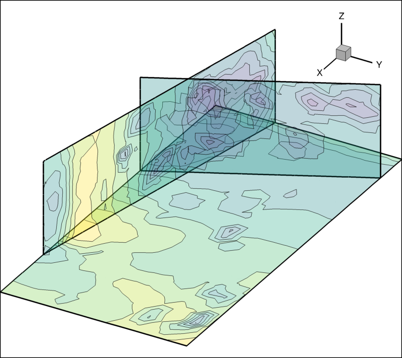
Up to eight different slice groups can be set and each slice group can use different slice planes or different ranges for the same slice plane.
This class behaves like
SliceGroupexcept that setting any underlying style will do so for all of the represented slice groups. The style properties are then always returned as atupleof properties, one for each group, ordered by index number. This means there is an asymmetry between setting and getting any property under this object, illustrated by the following example:>>> slices = plot.slices(0, 1, 2) >>> slices.show = True >>> print(slices.show) (True, True, True)
All examples that set style on a single slice like the following:
>>> plot.slice(0).contour.show = True
may be converted to setting the same style on all slice groups like so:
>>> plot.slices().contour.show = True
See also
Added in version 1.2: Slice collection objects.
Attributes
Normal for arbitrary slices.
Orientation of data clipping for this slice group.
Contour attributes for the slice group.
Edge attributes for this slice group.
Effects attributes for this slice group.
Position of the end slice.
Mesh attributes for this slice group.
Number of intermediate slicing planes.
Obey source zone blanking.
Select on which plane the slice is drawn.
Origin of the slice.
Shade attributes for this slice group.
Show slices for this slice group.
Show intermediate slices.
bool; Include the primary slice (first slice placed) in the Plot.Include start and end slices.
SliceSource: Zones to slice through.Position of the start slice.
Determines how the surface is generated.
Clip this slice by any intersecting slices.
Vector attributes for this slice group.
Methods
extract([mode, assign_strand_ids, ...])Create new zones from this slice collection.
- SliceGroupCollection.arbitrary_normal
Normal for arbitrary slices.
Example usage:
>>> plot.slice(0).orientation = SliceSurface.Arbitrary
>>> plot.slice(0).arbitrary_normal = (0.1, 0.2, 0.3)
>>> plot.slice(0).arbitrary_normal.x
0.1
>>> plot.slice(0).arbitrary_normal.y
0.2
>>> plot.slice(0).arbitrary_normal.z
0.3
- Type:
- SliceGroupCollection.clip
Orientation of data clipping for this slice group.
Clipping the field data, isosurfaces, streamtraces or other plot objects using slices requires setting the
clipproperty of the slice as well as adding the slice group to theclip_planesproperty on the fieldmap effects. Only slice groups 0 to 5 are available for clipping in this framework:>>> from tecplot.constant import * >>> # setup slice and clipping orientation >>> slice = plot.slice(0) >>> slice.origin = (7, 0, 0) >>> slice.clip = ClipPlane.AbovePrimarySlice >>> # add slice group to the fieldmap clip planes >>> plot.fieldmap(0).effects.clip_planes = [slice] >>> # turn on and set value of isosurface >>> # and enforce slice clipping >>> isosurf = plot.isosurface(0) >>> isosurf.isosurface_values = 3 >>> isosurf.use_slice_clipping = True >>> # turn on isosurfaces and slices >>> pt.show_isosurfaces = True >>> pt.show_slices = True
Warning
Slice clipping is only supported for X, Y and Z-planes.
Slice clipping has no effect for slices that have an orientation of
SliceSurface.Arbitrary,SliceSurface.IPlanes,SliceSurface.JPlanesor ,SliceSurface.KPlanes. That is, the orientation must be one of:SliceSurface.XPlanes,SliceSurface.YPlanesorSliceSurface.ZPlanes.- Type:
- SliceGroupCollection.contour
Contour attributes for the slice group.
Example usage:
>>> plot.slice(0).contour.show = True
- Type:
- SliceGroupCollection.edge
Edge attributes for this slice group.
Example usage:
>>> plot.slice(0).edge.show = True
- Type:
- SliceGroupCollection.effects
Effects attributes for this slice group.
Example usage:
>>> plot.slice(0).effects.use_translucency = True
- Type:
- SliceGroupCollection.end_position
Position of the end slice.
SliceGroup.show_start_and_end_slicesmust beTrueto show the end slice. This will be a 3-tupleoffloatiforientationisX,Y,Zor zero-basedintiforientationisI,J,K.Example usage:
>>> plot.slice(0).show_start_and_end_slices = True
>>> plot.slice(0).end_position = (1, 1, 1)
>>> plot.slice(0).end_position.i
1
- SliceGroupCollection.extract(mode=ExtractMode.SingleZone, assign_strand_ids=True, resulting_1d_zone_type=Resulting1DZoneType.IOrderedIfPossible, transient_mode=TransientOperationMode.SingleSolutionTime)[source]
Create new zones from this slice collection.
Extracts the current slices represented by this group to the
Datasetas one or more zones.- Parameters:
mode (
ExtractMode, optional) – Determines how many zones are created upon extraction. Possible values are:ExtractMode.SingleZone(default) andExtractMode.OneZonePerConnectedRegion.assign_strand_ids (
bool, optional) – Automatically assign strand ID’s to the created zones. (default:True)resulting_1d_zone_type (
Resulting1DZoneType, optional) – The type of zone to create when the result is one-dimensional. Possible values are:Resulting1DZoneType.IOrderedIfPossible(default) andResulting1DZoneType.FELineSegment.transient_mode (
TransientOperationMode) – Determines which solution times are used to extract slices when transient data is available in the dataset. Possible values areTransientOperationMode.SingleSolutionTime(default) orTransientOperationMode.AllSolutionTimes.
- Returns:
generator of the extracted zones.
See also
Example usage showing how to convert the resulting generator into a reusable list object of zones:
>>> slice_zones = list(plot.slices(0, 1).extract())
- SliceGroupCollection.indices
- SliceGroupCollection.mesh
Mesh attributes for this slice group.
Example usage:
>>> plot.slice(0).mesh.show = True
- Type:
- SliceGroupCollection.num_intermediate_slices
Number of intermediate slicing planes.
You may specify between 1 and 5,000 intermediate slices.
Example usage:
>>> # Show 2 intermediate slices
>>> plot.slice(0).num_intermediate_slices = 2
- Type:
- SliceGroupCollection.obey_source_zone_blanking
Obey source zone blanking.
When set to
True, slices are subject to any blanking used for the data. When set toFalse, slices are generated for blanked and unblanked regions.Example usage:
>>> plot.slice(0).obey_source_zone_blanking = True
- Type:
- SliceGroupCollection.orientation
Select on which plane the slice is drawn.
You may also choose
SliceSurface.Arbitraryto place the slice on an arbitrary plane.To orient slices in an arbitrary direction, choose
SliceSurface.Arbitrary. As with other slices, you may specify origin points for a primary slice and/or for start and end slices. Slices pass through the indicated origin point(s), so you can easily align the edge of a slice or group of slices along some other feature of the plot, such as an axis. If intermediate slices are activated, they are drawn equally spaced between the slices defined by the start and end origins.Example usage:
>>> plot.slice(0).orientation = SliceSurface.XPlanes
- Type:
- SliceGroupCollection.origin
Origin of the slice.
This will be a 3-
tupleoffloatiforientationisX,Y,Zor zero-basedintiforientationisI,J,K. For arbitrary slice orientation, the origin can be any location. For axis orientations (XPlanes,YPlanes, etc.) two of the three components are not used.Example usage:
>>> slice_0 = plot.slice(0)
>>> slice_0.orientation = SliceSurface.IPlanes
>>> slice_0.origin = (1, 0, 0)
>>> dx = (1, 1, 1)
>>> slice_0.origin += dx
>>> slice_0.origin.i
2
>>> slice_0.origin.j
1
>>> slice_0.origin.k
1

>>> slice_0.orientation = SliceSurface.Arbitrary
>>> slice_0.origin = (.5, .1, .1)
>>> slice_0.origin += dx
>>> slice_0.origin.x
1.5
>>> slice_0.origin.y
.1
>>> slice_0.origin.z
.1
- SliceGroupCollection.shade
Shade attributes for this slice group.
Example usage:
>>> plot.slice(0).shade.show = True
- Type:
- SliceGroupCollection.show
Show slices for this slice group.
Example usage:
>>> plot.slice(0).show = True
- Type:
- SliceGroupCollection.show_intermediate_slices
Show intermediate slices.
Intermediate slices are evenly distributed between the start and end slices.
Example usage:
>>> plot.slice(0).show_intermediate_slices = True
- SliceGroupCollection.show_primary_slice
bool; Include the primary slice (first slice placed) in the Plot.Example usage:
>>> plot.slice(0).show = True
>>> plot.slice(0).show_primary_slice = True
- SliceGroupCollection.show_start_and_end_slices
Include start and end slices.
Example usage:
>>> plot.slice(0).show_start_and_end_slices = True
- Type:
- SliceGroupCollection.slice_source
SliceSource: Zones to slice through.Choose to slice through volume Zones, surface Zones, or the surfaces of volume Zones.
Example usage:
>>> plot.slice(0).slice_source = SliceSource.SurfaceZones
- SliceGroupCollection.start_position
Position of the start slice.
SliceGroup.show_start_and_end_slicesmust beTrueto show the start slice. This will be a 3-tupleoffloatiforientationisX,Y,Zor zero-basedintiforientationisI,J,K.Example usage:
>>> plot.slice(0).show_start_and_end_slices = True
>>> plot.slice(0).start_position = (1, 1, 1)
>>> plot.slice(0).start_position.i
1
- SliceGroupCollection.surface_generation_method
Determines how the surface is generated.
May be one of:
SurfaceGenerationMethod.Auto:Selects one of the surface generation algorithms best suited for the zones participating in the slice generation. “All polygons” is used if one or more of the participating zones is polytope, otherwise “allow quads” is used.
SurfaceGenerationMethod.AllPolygons:Similar to the “All triangles” method except that all interior faces generated as a result of triangulation that are not part of the original mesh are eliminated. This preserves the original mesh of the source zones on the resulting slice.
SurfaceGenerationMethod.AllTriangles:An advanced algorithm that can handle complex saddle issues and guarantees that there will be no holes in the final surface. As the surface is composed entirely of triangles, it can be delivered more efficiently to the graphics hardware.
SurfaceGenerationMethod.AllowQuads:Produces quads or triangles, and the resulting surface more closely resembles the shape of the volume cells from the source zone. Since the quads are not arbitrarily divided into triangles, no biases are introduced, and the resulting surface may appear smoother. This method is preferred when the source zone is FE-Brick or IJK-Ordered and the surface is aligned with the source cells.
Example usage:
>>> from tecplot.constant import SurfaceGenerationMethod
>>> plot.slice(0).surface_generation_method = \
...     SurfaceGenerationMethod.AllowQuads
- Type:
- SliceGroupCollection.use_slice_clipping
Clip this slice by any intersecting slices.
Example usage:
>>> from tecplot.constant import ClipPlane
>>> slice = plot.slice(0)
>>> slice.clip = ClipPlane.AbovePrimarySlice
>>> plot.fieldmap(0).effects.clip_planes = slice
>>> plot.slice(1).use_slice_clipping = True
See also
- Type:
- SliceGroupCollection.vector
Vector attributes for this slice group.
Example usage:
>>> plot.slice(0).vector.show = True
- Type:
SliceContour
- class tecplot.plot.SliceContour(slice_group)[source]
Contour attributes of the slice group.
from os import path
import tecplot as tp
from tecplot.constant import SliceSurface, ContourType

examples_dir = tp.session.tecplot_examples_directory()
datafile = path.join(examples_dir, 'SimpleData', 'DuctFlow.plt')
dataset = tp.data.load_tecplot(datafile)

plot = tp.active_frame().plot()

plot.show_slices = True
slice_0 = plot.slice(0)

# Use contour(0) for Flooding and contour(2) for Lines
plot.contour(0).variable = dataset.variable('P(N/m2)')
plot.contour(2).variable = dataset.variable('T(K)')
plot.contour(2).legend.show = False
slice_0.contour.show = True
slice_0.contour.flood_contour_group = plot.contour(0)
slice_0.contour.line_contour_group = plot.contour(2)
slice_0.contour.contour_type = ContourType.Overlay  # AKA "Both lines and flood"

slice_0.show_primary_slice = False
slice_0.show_start_and_end_slices = True
slice_0.show_intermediate_slices = True
slice_0.start_position = (-.21, .05, .025)
slice_0.end_position = (1.342, .95, .475)
slice_0.num_intermediate_slices = 3

# ensure consistent output between interactive (connected) and batch
slice_0.contour.flood_contour_group.levels.reset_to_nice()
slice_0.contour.line_contour_group.levels.reset_to_nice()

tp.export.save_png('slice_contour.png', 600, supersample=3)

Attributes
Contour type for the slice contours.
Contour group to use for flooding.
Zero-based
Indexof the floddingContourGroup.Colorof contour lines.Contour group to use for contour lines.
Zero-based
Indexof theContourGroupfor contour lines.Contour line thickness as a percentage of frame width.
Show contours on the slice.
bool; Enable lighting effect.
- SliceContour.contour_type
Contour type for the slice contours.
Example usage:
>>> plot.show_slices = True >>> plot.slice(0).contour.contour_type = ContourType.AverageCell
- Type:
- SliceContour.flood_contour_group
Contour group to use for flooding.
Changing style on this
ContourGroupwill affect all fieldmaps on the sameFramethat use it.Example usage:
>>> group = plot.contour(1) >>> contour = plot.slice(1).contour >>> contour.flood_contour_group = group
- Type:
- SliceContour.flood_contour_group_index
Zero-based
Indexof the floddingContourGroup.This property sets and gets, by
Index, theContourGroupused for flooding. Changing style on thisContourGroupwill affect all fieldmaps on the sameFramethat use it.Example usage:
>>> plot.show_slices = True >>> contour = plot.slice(0).contour >>> contour.flood_contour_group_index = 1
- Type:
- SliceContour.line_color
Colorof contour lines.Selecting
Color.MultiColorwill color the slice contour lines based on thecontour groupvariable.Example usage:
>>> plot.show_slices = True >>> plot.slice(0).contour.line_color = Color.Blue
- Type:
- SliceContour.line_contour_group
Contour group to use for contour lines.
Changing style on this
ContourGroupwill affect all fieldmaps on the sameFramethat use it.Example usage:
>>> group = plot.contour(1) >>> contour = plot.slice(1).contour >>> contour.line_contour_group = group
- Type:
- SliceContour.line_contour_group_index
Zero-based
Indexof theContourGroupfor contour lines.This property sets and gets, by
Index, theContourGroupused for line placement. Although all properties of theContourGroupcan be manipulated through this object, many of them (i.e., color) will not affect the lines unless theFieldmapContour.line_coloris set to the sameContourGroup. Note that changing style on thisContourGroupwill affect all other fieldmaps on the sameFramethat use it.Example usage:
>>> plot.show_slices = True >>> contour = plot.slice(0).contour >>> contour.line_contour_group_index = 2
- Type:
- SliceContour.line_thickness
Contour line thickness as a percentage of frame width.
Suggested values are one of: .02, .1, .4, .8, 1.5
Example usage:
>>> plot.show_slices = True >>> plot.slice(0).contour.line_thickness = .4
- Type:
- SliceContour.show
Show contours on the slice.
Example usage:
>>> plot.show_slices = True >>> plot.slice(1).contour.show = True
- Type:
- SliceContour.use_lighting_effect
bool; Enable lighting effect.Note
Setting
SliceContour.use_lighting_effectwill also set the same value forSliceShade.use_lighting_effect, and vice-versa.The lighting effect is set with
SliceEffects.lighting_effect, and may be one ofLightingEffect.SmoothWithCreases,LightingEffect.Smooth, orLightingEffect.Paneled.Example usage:
>>> plot.show_slices = True >>> contour = plot.slice(0).contour >>> contour.use_lighting_effect = True >>> plot.slice(0).effects.lighting_effect = LightingEffect.Paneled
SliceEdge
- class tecplot.plot.SliceEdge(slice_group)[source]
Edge attributes of the slice group.
When enabled, selected edge lines of all slices in this group will be shown:
from os import path import tecplot as tp examples_dir = tp.session.tecplot_examples_directory() datafile = path.join(examples_dir, 'SimpleData', 'DuctFlow.plt') dataset = tp.data.load_tecplot(datafile) plot = tp.active_frame().plot() plot.show_slices = True plot.contour(0).variable = dataset.variable('U(M/S)') slice_0 = plot.slice(0) slice_0.edge.show = True slice_0.edge.line_thickness = 0.8 # ensure consistent output between interactive (connected) and batch plot.contour(0).levels.reset_to_nice() tp.export.save_png('slice_edge.png', 600, supersample=3)
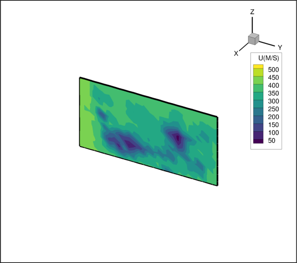
Attributes
Edge color.
Edge type.
Edge line thickness as a percentage of frame width.
Show edges.
- SliceEdge.color
Edge color.
Example usage:
>>> plot.slice(0).edge.show = True >>> plot.slice(0).edge.color = Color.Blue
- Type:
- SliceEdge.edge_type
Edge type.
There are two types of edges in Tecplot 360: creases and borders.
An edge border is the boundary of a Zone. An edge crease appears when the inside angle between two cells is less than a user-defined limit. The inside angle can range from 0-180 degrees (where 180 degrees indicates coplanar surfaces). The default inside angle for determining an edge crease is 135 degrees.
Example usage:
>>> plot.slice(0).edge.show = True >>> plot.slice(0).edge.edge_type = EdgeType.BordersAndCreases
- Type:
- SliceEdge.line_thickness
Edge line thickness as a percentage of frame width.
Example usage:
>>> plot.slice(0).edge.show = True >>> plot.slice(0).edge.line_thickness = .8
- Type:
SliceEffects
- class tecplot.plot.SliceEffects(slice_group)[source]
Slice effects for this slice.
from os import path import tecplot as tp examples_dir = tp.session.tecplot_examples_directory() datafile = path.join(examples_dir, 'SimpleData', 'DuctFlow.plt') dataset = tp.data.load_tecplot(datafile) plot = tp.active_frame().plot() plot.show_slices = True slice_0 = plot.slice(0) plot.contour(0).variable = dataset.variable('U(M/S)') slice_0.contour.show = True slice_0.effects.use_translucency = True slice_0.effects.surface_translucency = 70 # ensure consistent output between interactive (connected) and batch plot.contour(0).levels.reset_to_nice() tp.export.save_png('slice_effects.png', 600, supersample=3)

Attributes
Surface lighting effect.
Surface translucency of the slice group.
Enable surface translucency for this slice group.
- SliceEffects.lighting_effect
Surface lighting effect.
Slice lighting effects must be enabled by setting
SliceContour.use_lighting_effectorSliceShade.use_lighting_effecttoTruewhen setting this value.There are three types of lighting effects: Paneled, SmoothWithCreases and Smooth:
Paneled: Within each cell, the color assigned to each area byshading or contour flooding is tinted by a shade constant across the cell. This shade is based on the orientation of the cell relative to your 3D light source.
SmoothUnlike
Paneledshading that colors the cell surface considering a constant angle to the light relative to the cell’s surface normal,Smoothcomputes the average normal around each cell node and interpolates the lighting influence smoothly across the cell face.SmoothWithCreasesshading is not continuous across zone boundaries unless face neighbors are specified in the data.
SmoothWithCreasesThis option is similar to
Smoothbut considers the crease angle between neighboring, connected cell faces. When the crease angle exceeds the specified amount the edge is considered creased and the lighting interpolation across the cell uses the cell’s surface normal for the shared nodes along that edge instead of the average surface normal at those nodes. If the surface has many edges that exceed the crease angle, such as a very chaotic iso-surface, a significantly larger amount of data is required to render the surface.
Example usage:
>>> plot.slice(0).contour.use_lighting_effect = True >>> plot.slice(0).effects.lighting_effect = LightingEffect.Paneled
- Type:
- SliceEffects.surface_translucency
Surface translucency of the slice group.
Slice surface translucency must be enabled by setting
SliceEffects.use_translucency=Truewhen setting this value.Valid slice translucency values range from one (opaque) to 99 (translucent).
Example usage:
>>> plot.slice(0).effects.use_translucency = True >>> plot.slice(0).effects.surface_translucency = 20
- Type:
- SliceEffects.use_translucency
Enable surface translucency for this slice group.
The surface translucency value can be changed by setting
SliceEffects.surface_translucency.Example usage:
>>> plot.slice(0).effects.use_translucency = True >>> plot.slice(0).effects.surface_translucency = 20
- Type:
SliceMesh
- class tecplot.plot.SliceMesh(slice_group)[source]
Mesh attributes of the slice group.
from os import path import tecplot as tp from tecplot.constant import SliceSurface, ContourType examples_dir = tp.session.tecplot_examples_directory() datafile = path.join(examples_dir, 'SimpleData', 'DuctFlow.plt') dataset = tp.data.load_tecplot(datafile) plot = tp.active_frame().plot() plot.show_slices = True plot.contour(0).variable = dataset.variable('U(M/S)') plot.slice(0).mesh.show = True # ensure consistent output between interactive (connected) and batch plot.contour(0).levels.reset_to_nice() tp.export.save_png('slice_mesh.png', 600, supersample=3)
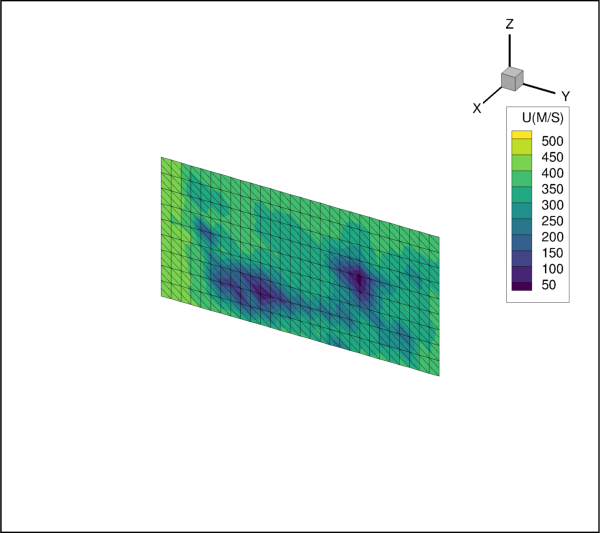
Attributes
Slice mesh line Color.
Mesh line thickness.
Show mesh lines.
- SliceMesh.color
Slice mesh line Color.
Slice mesh lines can be a solid color or be colored by a
ContourGroupas obtained through theplot.contourproperty.Example usage:
>>> plot.slice(0).mesh.show = True >>> plot.slice(0).mesh.color = Color.Green
- Type:
- SliceMesh.line_thickness
Mesh line thickness.
The mesh line thickness is specified as a percentage of the frame width.
Example usage:
>>> plot.slice(0).mesh.show = True >>> plot.slice(0).mesh.line_thickness = 0.8
- Type:
SliceShade
- class tecplot.plot.SliceShade(slice_group)[source]
Shade attributes of the slice group.
Show shading on the slice when
SliceContour.showhas not been selected or is set toContourType.Lines:from os import path import tecplot as tp from tecplot.constant import Color examples_dir = tp.session.tecplot_examples_directory() datafile = path.join(examples_dir, 'SimpleData', 'Pyramid.plt') dataset = tp.data.load_tecplot(datafile) plot = tp.active_frame().plot() plot.show_slices = True plot.slice(0).contour.show = False shade = plot.slice(0).shade shade.show = True shade.color = Color.Red # Slice will be colored solid red. tp.export.save_png('slice_shade.png', 600, supersample=3)
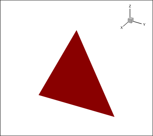
Attributes
Shade color.
Show shade attributes.
Use lighting effect.
- SliceShade.color
Shade color.
Color.MultiColorandColor.RGBColorcoloring are not available. Use flooded contours for multi-color or RGB floodingExample usage:
>>> plot.slice(0).shade.show = True >>> plot.slice(0).shade.color = Color.Blue
- Type:
- SliceShade.show
Show shade attributes.
Example usage:
>>> plot.slice(0).shade.show = True
- Type:
- SliceShade.use_lighting_effect
Use lighting effect.
When set to
True, the lighting effect may be selected with theSliceEffects.lighting_effectattribute.Note
Setting
SliceShade.use_lighting_effectwill also set the same value forSliceContour.use_lighting_effect, and vice-versa.Example usage:
>>> plot.slice(0).shade.use_lighting_effect = True >>> plot.slice(0).effects.lighting_effect = LightingEffect.Paneled
- Type:
SliceVector
- class tecplot.plot.SliceVector(slice_group)[source]
Vector attributes of the slice group.
from os import path import tecplot as tp from tecplot.constant import * examples_dir = tp.session.tecplot_examples_directory() datafile = path.join(examples_dir, 'SimpleData', 'DuctFlow.plt') dataset = tp.data.load_tecplot(datafile) plot = tp.active_frame().plot() plot.show_slices = True slice_0 = plot.slice(0) plot.contour(0).variable = dataset.variable('T(K)') # Vector variables must be assigned before displaying vectors = plot.vector vectors.u_variable = dataset.variable('U(M/S)') vectors.v_variable = dataset.variable('V(M/S)') vectors.w_variable = dataset.variable('W(M/S)') slice_vector = plot.slice(0).vector slice_vector.show = True slice_vector.vector_type = VectorType.MidAtPoint slice_vector.color = Color.BluePurple slice_0.effects.use_translucency = True slice_0.effects.surface_translucency = 30 # ensure consistent output between interactive (connected) and batch plot.contour(0).levels.reset_to_nice() tp.export.save_png('slice_vector.png', 600, supersample=3)
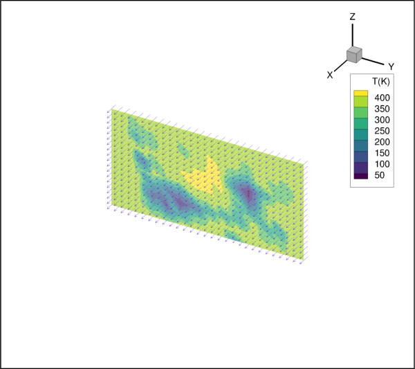
Attributes
Arrowhead style of slice vectors.
Set slice vector color.
Use tangent vectors for slices.
Vector line thickness as a percentage of the frame height.
Show vectors on slices.
Type of vector for slices in this slice group.
- SliceVector.arrowhead_style
Arrowhead style of slice vectors.
Example usage:
>>> plot.slice(0).vector.show = True >>> plot.slice(0).vector.arrowhead_style = ArrowheadStyle.Hollow
- Type:
- SliceVector.color
Set slice vector color.
Example usage:
>>> plot.slice(0).vector.show = True >>> plot.slice(0).vector.color = Color.Red
- Type:
- SliceVector.is_tangent
Use tangent vectors for slices.
Example usage:
>>> plot.slice(0).vector.show = True >>> plot.slice(0).vector.is_tangent = True
- Type:
- SliceVector.line_thickness
Vector line thickness as a percentage of the frame height.
Typical values are .02, .1, .4, .8, 1.5
Example usage:
>>> plot.slice(0).vector.show = True >>> plot.slice(0).vector.line_thickness = .1
- Type:
- SliceVector.show
Show vectors on slices.
Example usage:
>>> plot.slice(0).vector.show = True
- Type:
- SliceVector.vector_type
Type of vector for slices in this slice group.
Example usage:
>>> plot.slice(0).vector.show = True >>> plot.slice(0).vector.vector_type = VectorType.MidAtPoint
- Type:
Streamtraces
Streamtraces
- class tecplot.plot.Streamtraces(plot)[source]
Streamtrace attributes for the plot.
A streamtrace is the path traced by a massless particle placed at an arbitrary location in a steady-state vector field. Streamtraces may be used to illustrate the nature of the vector field flow in a particular region of the Plot.
Note
Because streamtraces are dependent upon a vector field, you must define vector components before creating streamtraces. However, it is not necessary to activate the Vector zone layer to use streamtraces.
import os import tecplot from tecplot.constant import * examples_dir = tecplot.session.tecplot_examples_directory() datafile = os.path.join(examples_dir, 'SimpleData', 'Eddy.plt') dataset = tecplot.data.load_tecplot(datafile) frame = tecplot.active_frame() frame.plot_type = tecplot.constant.PlotType.Cartesian3D plot = frame.plot() plot.fieldmap(0).surfaces.surfaces_to_plot = SurfacesToPlot.BoundaryFaces plot.show_mesh = True plot.show_shade = False plot.vector.u_variable_index = 4 plot.vector.v_variable_index = 5 plot.vector.w_variable_index = 6 plot.show_streamtraces = True streamtraces = plot.streamtraces streamtraces.color = Color.Blue streamtraces.show_arrows = True streamtraces.arrowhead_size = 2 streamtraces.step_size = .25 streamtraces.line_thickness = .2 streamtraces.max_steps = 100 streamtraces.add_rake(start_position=(45.49, 15.32, 59.1), end_position=(48.89, 53.2, 47.6), stream_type=Streamtrace.SurfaceLine, num_seed_points=4) tecplot.export.save_png('streamtrace_example.png', 600, supersample=3)
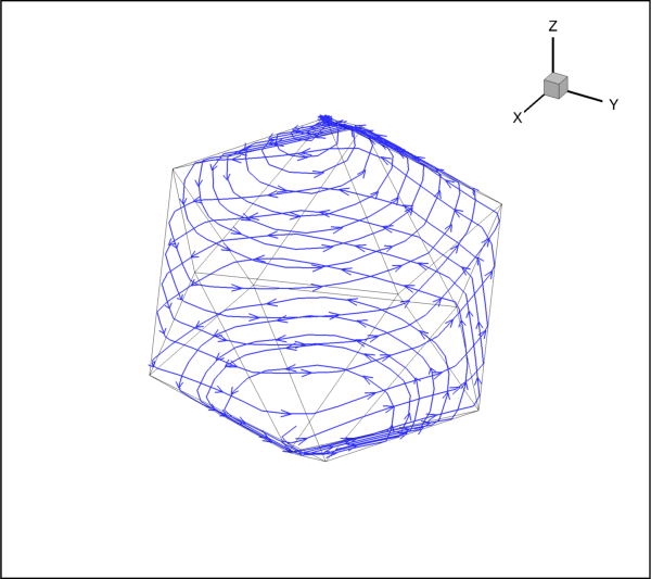
Attributes
Determine if there are active streamtraces.
Arrowhead size as a percentage of frame height.
Distance between arrowheads in terms of Y-frame units.
Color of streamtraces line (not rods or ribbons).
Query the number of active streamtraces for the current plot type.
Number of time deltas used for the "off" sections of the streamlines.
Determine if the streamtraces have the terminating line.
Streamtrace line thickness.
Colorof the streamline markers.Size of streamline markers.
The
SymbolTypeto use for stream markers.Maximum number of steps before the streamtrace is terminated.
Smallest step size to use as a percentage of cell distance.
Obey source zone blanking.
Streamtrace rod/ribbon attributes.
Display arrowheads along all streamlines.
Display streamtrace dashes.
Display streamtrace markers.
Draw streamtrace paths (lines, ribbons, or rods).
Maximum fraction of the distance across a cell that a streamtrace moves in one step.
Streamtraces termination line attributes.
Streamtraces timing attributes.
Clip isosurface by any intersecting slices.
Methods
add(seed_point, stream_type[, direction])Add a single streamtrace to the plot of the current frame.
add_on_zone_surface(stream_type[, zones, ...])Add streamtraces to one or more zones in a plot.
add_rake(start_position, end_position, ...)Add a rake of streamtraces to the plot of the current frame.
Delete all streamtraces for the current plot type.
delete_range(range_start, range_end)Delete a range of streamtraces.
extract([concatenate, assign_strand_ids])Create new zones from streamtraces
marker_symbol([symbol_type])Returns a streamline symbol style object.
position(stream_number)Query the starting position of a streamtrace.
set_termination_line(line_points)Set the position of the termination line for streamtraces.
streamtrace_type(stream_number)Query the type of a streamtrace by streamtrace number.
- Streamtraces.active
Determine if there are active streamtraces.
Note
This property is read-only.
Example usage:
>>> streamtraces_are_active = plot.streamtraces.active
- Type:
- Streamtraces.add(seed_point, stream_type, direction=StreamDir.Both)[source]
Add a single streamtrace to the plot of the current frame.
The plot type must be either
Cartesian2DorCartesian3D.- Parameters:
seed_point – (2- or 3-
tupleoffloats): Pass a 2-tupleoffloatfor aCartesian2DFieldPlot, or a 3-tupleoffloatfor aCartesian3DFieldPlot.stream_type – (
Streamtrace): Type of streamtraces to add.direction – (
StreamDir, optional): Direction of propagation of the streamtraces being added.
Note
stream_type is automatically set to
Streamtrace.SurfaceLineif the plot type isCartesian2DFieldPlot. The only stream type available for 2D plots isStreamtrace.SurfaceLine.import os import tecplot from tecplot.constant import * import numpy as np examples_dir = tecplot.session.tecplot_examples_directory() datafile = os.path.join(examples_dir, 'SimpleData', 'DuctFlow.plt') dataset = tecplot.data.load_tecplot(datafile) frame = tecplot.active_frame() frame.plot_type = tecplot.constant.PlotType.Cartesian3D plot = frame.plot() plot.contour(0).variable = dataset.variable('P(N/m2)') plot.contour(0).levels.reset_to_nice() plot.contour(0).legend.show = False plot.vector.u_variable = dataset.variable('U(M/S)') plot.vector.v_variable = dataset.variable('V(M/S)') plot.vector.w_variable = dataset.variable('W(M/S)') # Goal: create a grid of 12 stream trace ribbons x_slice_location = .79 y_start = .077 y_end = .914 z_start = .052 z_end = .415 num_left_right_slices = 4 # Must be >= 2 num_top_bottom_slices = 3 # Must be >= 2 plot.show_streamtraces = True streamtraces = plot.streamtraces streamtraces.show_paths = True rod = streamtraces.rod_ribbon rod.width = .03 rod.contour.show = True for y in np.linspace(y_start, y_end, num=num_left_right_slices): for z in np.linspace(z_start, z_end, num=num_top_bottom_slices): streamtraces.add([x_slice_location,y,z], Streamtrace.VolumeRibbon) tecplot.export.save_png('streamtrace_add_xyz.png', 600, supersample=3)
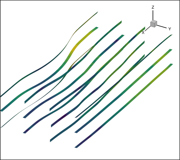
- Streamtraces.add_on_zone_surface(stream_type, zones=None, num_seed_points=10, direction=StreamDir.Both)[source]
Add streamtraces to one or more zones in a plot.
The plot type must be either
Cartesian2DorCartesian3D.Note
For volume zones the streamtraces are propagated from the surfaces of the volume.
- Parameters:
stream_type – (
Streamtrace): Type of streamtraces to add.zones (
setofintegers, optional) – Set of Zones on which to add streamtraces. IfNone, then streamtraces will be added to the currently active zones.num_seed_points – (
int, optional): Number of seed points for distributing along a rake or on defined surfaces.direction – (
StreamDir, optional): Direction of propagation of the streamtraces being added.
import os import tecplot from tecplot.constant import * examples_dir = tecplot.session.tecplot_examples_directory() datafile = os.path.join(examples_dir, 'OneraM6wing', 'OneraM6_SU2_RANS.plt') dataset = tecplot.data.load_tecplot(datafile) frame = tecplot.active_frame() frame.plot_type = tecplot.constant.PlotType.Cartesian3D plot = frame.plot() plot.vector.u_variable_index = 4 plot.vector.v_variable_index = 5 plot.vector.w_variable_index = 6 plot.show_streamtraces = True plot.streamtraces.add_on_zone_surface( # To add streamtraces to the currently active zones, # pass zones=None zones=[1], # Add streamtraces on 2nd zone only stream_type=Streamtrace.SurfaceLine, num_seed_points=200) tecplot.export.save_png('streamtrace_add_on_zone_surface.png', 600, supersample=3)
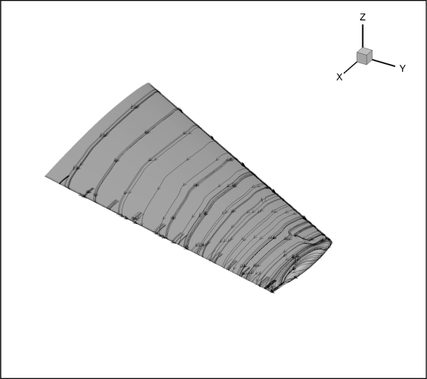
- Streamtraces.add_rake(start_position, end_position, stream_type, num_seed_points=10, direction=StreamDir.Both)[source]
Add a rake of streamtraces to the plot of the current frame.
The plot type must be either
Cartesian2DorCartesian3D.- Parameters:
start_position – (2- or 3-
tupleoffloats): Pass a 2-tupleoffloatfor aCartesian2DFieldPlot, or a 3-tupleoffloatfor aCartesian3DFieldPlot.end_position – (2- or 3-
tupleoffloats): Pass a 2-tupleoffloatfor aCartesian2DFieldPlot, or a 3-tupleoffloatfor aCartesian3DFieldPlot.stream_type – (
Streamtrace): Type of streamtraces to add.num_seed_points – (
int, optional): Number of seed points for distributing along a rake or on defined surfaces.direction – (
StreamDir, optional): Direction of propagation of the streamtraces being added.
import os import tecplot from tecplot.constant import * examples_dir = tecplot.session.tecplot_examples_directory() datafile = os.path.join(examples_dir, 'SimpleData', 'Eddy.plt') dataset = tecplot.data.load_tecplot(datafile) frame = tecplot.active_frame() frame.plot_type = tecplot.constant.PlotType.Cartesian3D plot = frame.plot() plot.fieldmap(0).surfaces.surfaces_to_plot = SurfacesToPlot.BoundaryFaces plot.show_mesh = True plot.show_shade = False plot.vector.u_variable_index = 4 plot.vector.v_variable_index = 5 plot.vector.w_variable_index = 6 plot.show_streamtraces = True streamtraces = plot.streamtraces streamtraces.add_rake(start_position=[.5, .5, .5], end_position=[20, 20, 20], stream_type=Streamtrace.VolumeLine) tecplot.export.save_png('streamtrace_add_rake.png', 600, supersample=3)
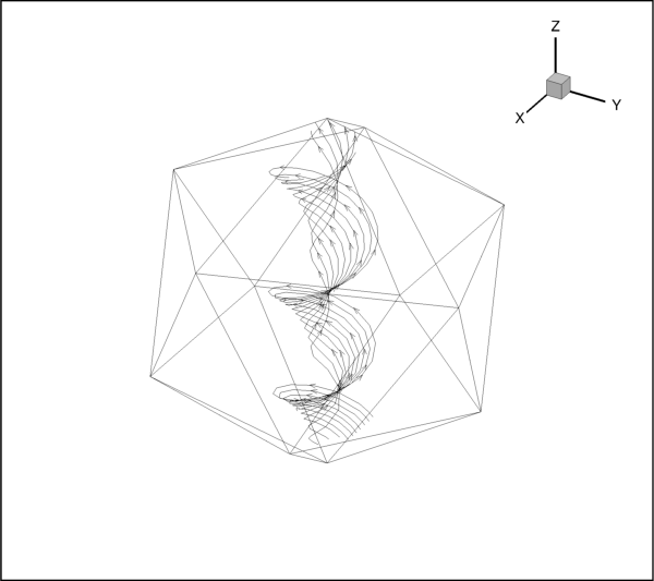
- Streamtraces.arrowhead_size
Arrowhead size as a percentage of frame height.
Recommend values are one of 1, 3, 5, 8, or 12.
Example usage:
>>> plot.streamtraces.show_arrows = True >>> plot.streamtraces.arrowhead_size = 1.0
- Type:
- Streamtraces.arrowhead_spacing
Distance between arrowheads in terms of Y-frame units.
For example, a value of 10 will space arrowheads approximately ten percent of the frame height apart from each other along each streamline.
Example usage:
>>> plot.streamtraces.show_arrows = True >>> plot.streamtraces.arrowhead_spacing = 10
- Type:
- Streamtraces.color
Color of streamtraces line (not rods or ribbons).
Streamtraces can be a solid color or be colored by a
ContourGroupas obtained through theplot.contourproperty.Example usage:
>>> plot.streamtraces.color = Color.Red
- Type:
- Streamtraces.count
Query the number of active streamtraces for the current plot type.
- Returns:
Note
This property is read-only.
>>> num_active_streamtraces = plot.streamtraces.count
- Streamtraces.dash_skip
Number of time deltas used for the “off” sections of the streamlines.
Note
The
dash_skipvalue must be greater than 0.Example usage:
>>> plot.streamtraces.dash_skip = 2
- Type:
- Streamtraces.delete_all()[source]
Delete all streamtraces for the current plot type.
2D and 3D streamtraces are independent of each other.
If the plot type is
Cartesian2D, all 2D streamtraces are deleted. If the plot type isCartesian3D, all 3D streamtraces are deleted.- Raises:
TecplotSystemError – The streamtraces could not be deleted.
Example usage:
>>> plot.streamtraces.delete_all()
- Streamtraces.delete_range(range_start, range_end)[source]
Delete a range of streamtraces.
- Parameters:
- Raises:
TecplotSystemError – The streamtraces in the range could not be deleted.
Example usage:
>>> # Delete the first 100 streamtraces >>> plot.streamtraces.delete_range(0, 99)
- Streamtraces.extract(concatenate=False, assign_strand_ids=True)[source]
Create new zones from streamtraces
Extracts the current streamtraces defined in this class to the
Datasetas one or more zones.- Parameters:
concatenate (
bool, optional) – Concatenate streamtraces into a single zone for each format (Surface Line, Volume Line, Volume Ribbon, Volume Rod).assign_strand_ids (
bool, optional) – Automatically assign strand ID’s to the created zones. This option is ignored if concatenate ifTrue. (default:True)
- Returns:
A generator of the extracted zones.
Example usage:
>>> slice_zone = plot.streamtraces.extract()
- Streamtraces.has_terminating_line
Determine if the streamtraces have the terminating line.
Note
This property is read-only.
Example usage:
>>> has_terminating_line = plot.streamtraces.has_terminating_line
- Streamtraces.line_thickness
Streamtrace line thickness.
Line thickness as a percentage of the frame height for 2D lines, or a percentage of the median axis length for 3D surface lines and volume lines.
Suggested values are .02, .1, .4, .8, 1.5
Example usage:
>>> plot.streamtraces.line_thickness = 1.1
- Type:
- Streamtraces.marker_color
Colorof the streamline markers.Streamtrace markers can be a solid color or be colored by a
ContourGroupas obtained through theplot.contourproperty.Example usage:
>>> plot.streamtraces.marker_color = Color.Blue
- Type:
- Streamtraces.marker_size
Size of streamline markers.
Example usage:
>>> plot.streamtraces.marker_size = 1.1
- Type:
- Streamtraces.marker_symbol(symbol_type=None)[source]
Returns a streamline symbol style object.
- Parameters:
symbol_type (
SymbolType, optional) – The type of symbol to return. By default, this will return the active marker symbol type which is obtained fromStreamtraces.marker_symbol_type.
Returns:
TextSymbolorGeometrySymbol, depending onmarker_symbol_typeExample usage:
>>> from tecplot.constant import SymbolType >>> streamtrace = plot.streamtraces >>> streamtraces.marker_symbol_type = SymbolType.Text >>> symbol = streamtraces.marker_symbol(SymbolType.Text) >>> symbol.text = 'a'
- Streamtraces.marker_symbol_type
The
SymbolTypeto use for stream markers.This sets the active symbol type for streamtrace markers. Use
Streamtraces.marker_symbolto access the symbol:>>> from tecplot.constant import SymbolType >>> streamtrace = plot.streamtraces >>> streamtraces.marker_symbol_type = SymbolType.Text >>> symbol = streamtraces.marker_symbol(SymbolType.Text) >>> symbol.text = 'a'
- Type:
- Streamtraces.max_steps
Maximum number of steps before the streamtrace is terminated.
max_stepsprevents streamtraces from spinning forever in a vortex, or from wandering into a region where the vector components are very small, very random, or both.If a small
step_sizeis selected, themax_stepsshould be a large value.Example usage:
>>> plot.streamtraces.max_steps = 5000
- Type:
- Streamtraces.min_step_size
Smallest step size to use as a percentage of cell distance.
A typical minimum step size value is 0.00001, which is the default.
Warning
Setting this too small results in integration problems. Setting this greater than or equal to the
step_sizeresults in a constant step size.Example usage:
>>> plot.streamtraces.min_step_size = .0002
- Type:
- Streamtraces.obey_source_zone_blanking
Obey source zone blanking.
When
True, streamtraces are generated for non-blanked regions only. WhenFalse, streamtraces are generated for both blanked and unblanked regions.Example usage:
>>> plot.streamtraces.obey_source_zone_blanking = True
- Type:
- Streamtraces.position(stream_number)[source]
Query the starting position of a streamtrace.
Get the position of streamtrace number 3:
>>> position = plot.streamtraces.position(2) # Note: 0-based >>> position.x # == position[0] 0.1 >>> position.y # == position[1] 0.2 >>> position.z # == position[2] 0.3
- Streamtraces.rod_ribbon
Streamtrace rod/ribbon attributes.
Example usage:
>>> streamtraces.rod_ribbon.mesh.show = True
- Type:
- Streamtraces.set_termination_line(line_points)[source]
Set the position of the termination line for streamtraces.
- Parameters:
line_points – (array of
floattuple) Points of the termination line.- Raises:
TecplotSystemError – Termination line could not be set.
Example usage:
>>> # Multi-segment line between points (0,0)-(5,8)-(3,6) >>> line_points = [(0, 0), (5, 8), (3,6)] >>> plot.streamtraces.set_termination_line(line_points)
- Streamtraces.show_arrows
Display arrowheads along all streamlines.
Example usage:
>>> plot.streamtraces.show_arrows = True
- Type:
- Streamtraces.show_dashes
Display streamtrace dashes.
The lengths of the dashes and the spaces between the dashes are controlled by the value of
StreamtraceTiming.delta. Set theStreamtraces.dash_skipattribute to control the number of time deltas used for the “off” sections of the streamtraces.Example usage:
>>> plot.streamtraces.show_dashes = True
- Type:
- Streamtraces.show_markers
Display streamtrace markers.
Stream markers are only available for surface and volume type streamlines.
You may also specify the
size,color, andshapeof the markers.Example usage:
>>> plot.streamtraces.show_markers = True
- Type:
- Streamtraces.show_paths
Draw streamtrace paths (lines, ribbons, or rods).
A streamtrace path may be a line, ribbon or rod.
Example usage:
>>> plot.streamtraces.show_paths = True
See also
Streamtraces.show_markers- Type:
- Streamtraces.step_size
Maximum fraction of the distance across a cell that a streamtrace moves in one step.
The step size is the maximum fraction of the distance across a cell that a streamtrace moves in one step. A streamtrace adjusts its step size between
step_sizeandmin_step_size, depending on local curvature of the streamtrace.A typical value (and the default) is 0.25, which results in four integration steps through each cell or element. The value for Step Size affects the accuracy of the integration.
Warning
Setting step size too small can result in round-off errors, while setting it too large can result in truncation errors and missed cells.
Example usage:
>>> plot.streamtraces.step_size = .25
- Type:
- Streamtraces.streamtrace_type(stream_number)[source]
Query the type of a streamtrace by streamtrace number.
- Parameters:
stream_number – (
int): 0-based stream number to query.- Returns:
Get the type of streamtrace 3. Note 0-based stream number:
>>> streamtrace_type = plot.streamtraces.streamtrace_type(2) >>> streamtrace_type <Streamtrace.VolumeLine: 2>
- Streamtraces.termination_line
Streamtraces termination line attributes.
A streamtrace termination line is a polyline that terminates any streamtraces that cross it. The termination line is useful for stopping streamtraces before they spiral or stall.
Example usage:
>>> term_line = plot.streamtraces.termination_line >>> term_line.show = True
- Streamtraces.timing
Streamtraces timing attributes.
Example usage:
>>> timing = plot.streamtraces.timing >>> timing.start = 0.01
- Type:
- Streamtraces.use_slice_clipping
Clip isosurface by any intersecting slices.
Example usage:
>>> from tecplot.constant import ClipPlane >>> slice = plot.slice(0) >>> slice.clip = ClipPlane.AbovePrimarySlice >>> plot.fieldmap(0).effects.clip_planes = slice >>> plot.streamtraces.use_slice_clipping = True
See also
- Type:
StreamtraceRodRibbon
- class tecplot.plot.StreamtraceRodRibbon(streamtrace)[source]
Get/Set streamtrace rod/ribbon attributes.
The
StreamtraceRodRibbonclass allows you to query and set attributes of streamtrace rod/ribbon types:In addition to attributes common to all rod/ribbon streamtrace types such as
width, some attributes are further divided into subcategories:Note
To change the color of streamtrace rods/ribbons, set
StreamtraceRodRibbonShade.color.import os import tecplot from tecplot.constant import * examples_dir = tecplot.session.tecplot_examples_directory() datafile = os.path.join(examples_dir, 'SimpleData', 'DuctFlow.plt') dataset = tecplot.data.load_tecplot(datafile) frame = tecplot.active_frame() frame.plot_type = tecplot.constant.PlotType.Cartesian3D plot = frame.plot() plot.show_mesh = False plot.show_shade = False plot.show_edge = True plot.fieldmap(0).edge.edge_type = EdgeType.Creases plot.contour(0).variable = dataset.variable(3) plot.contour(0).levels.reset_to_nice() plot.vector.u_variable_index = 3 plot.vector.v_variable_index = 4 plot.vector.w_variable_index = 5 plot.show_streamtraces = True plot.streamtraces.rod_ribbon.width = .03 plot.streamtraces.rod_ribbon.contour.show = True plot.streamtraces.add_rake(start_position=(1.5, 0.1, .4), end_position=(1.5, .9, 0.1), stream_type=Streamtrace.VolumeRibbon, num_seed_points=3) plot.streamtraces.add_rake(start_position=(1.5, 0.1, 0.1), end_position=(1.5, .9, .4), stream_type=Streamtrace.VolumeRod, num_seed_points=4) tecplot.export.save_png('streamtrace_ribbon.png', 600, supersample=3)
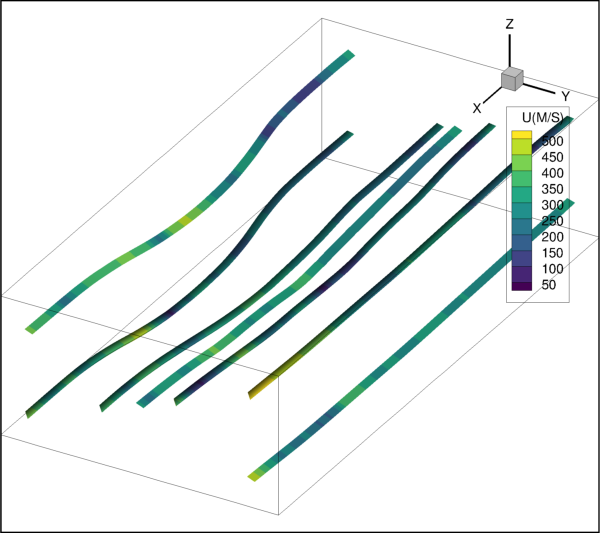
Attributes
Streamtraces rod/ribbon contour attributes.
Streamtraces rod/ribbon effects.
Streamtraces rod/ribbon mesh attributes.
Number of rod points.
Streamtraces rod/ribbon color and lighting attributes.
Rod/ribbon width in grid units.
- StreamtraceRodRibbon.contour
Streamtraces rod/ribbon contour attributes.
Example usage:
>>> plot.streamtraces.rod_ribbon.contour.show = True
- StreamtraceRodRibbon.effects
Streamtraces rod/ribbon effects.
Example usage:
>>> plot.streamtraces.rod_ribbon.effects.use_translucency = True
- StreamtraceRodRibbon.mesh
Streamtraces rod/ribbon mesh attributes.
Example usage:
>>> plot.streamtraces.rod_ribbon.mesh.show = True
- Type:
- StreamtraceRodRibbon.num_rod_points
Number of rod points.
Volume rods have a polygonal cross-section; this parameter tells Tecplot 360 what that cross-section should be. (Three is an equilateral triangle, four is a square, five is a regular pentagon, and so on.) If you want two sets of volume rods with different cross-sections, you must create one set and then extract the set as a zone, then configure a new set of streamtraces with the second cross-section.
Example usage:
>>> plot.streamtraces.rod_ribbon.num_rod_points = 10
- Type:
int, valid range 3-100
- StreamtraceRodRibbon.shade
Streamtraces rod/ribbon color and lighting attributes.
Example usage:
>>> plot.streamtraces.rod_ribbon.shade.color = Color.Magenta
StreamtraceTiming
- class tecplot.plot.StreamtraceTiming(streamtrace)[source]
Timed markers for streamlines.
Use
StreamtraceTimingto control timed markers for streamlines, and timed dashes for all types of streamtraces. Stream markers are drawn at time locations along streamlines. The spacing between stream markers is proportional to the magnitude of the local vector field:import tecplot from tecplot.constant import * import os examples_dir = tecplot.session.tecplot_examples_directory() datafile = os.path.join(examples_dir, 'SimpleData', 'VortexShedding.plt') dataset = tecplot.data.load_tecplot(datafile) frame = tecplot.active_frame() frame.plot_type = tecplot.constant.PlotType.Cartesian2D plot = frame.plot() plot.vector.u_variable = dataset.variable('U(M/S)') plot.vector.v_variable = dataset.variable('V(M/S)') plot.show_streamtraces = True plot.show_shade = True plot.fieldmap(0).shade.color = Color.LightBlue streamtraces = plot.streamtraces streamtraces.show_markers = True timing = streamtraces.timing timing.anchor = 0 timing.delta = 0.0001 streamtraces.marker_size = 1.5 streamtraces.marker_symbol().shape =GeomShape.RTri streamtraces.marker_color = Color.Mahogany streamtraces.add_rake(start_position=(-0.003, 0.005), end_position=(-0.003, -0.005), stream_type=Streamtrace.TwoDLine, num_seed_points=10) plot.axes.y_axis.min = -0.02 plot.axes.y_axis.max = 0.02 plot.axes.x_axis.min = -0.008 plot.axes.x_axis.max = 0.04 tecplot.export.save_png('streamtrace_timing.png', 600, supersample=3)
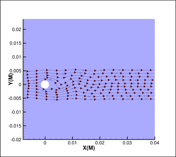
Attributes
Time that a dash is guaranteed to start.
Time between stream markers.
Time after which no stream markers are drawn.
Time at which the first marker should be drawn.
Methods
Reset the time delta for dashed streamtraces.
- StreamtraceTiming.anchor
Time that a dash is guaranteed to start.
A dash is guaranteed to start at
anchor, provided the start and end time surround the dash.Example usage:
>>> plot.streamtraces.timing.anchor = 1.1
- Type:
- StreamtraceTiming.delta
Time between stream markers.
deltais the time interval that measures the time between stream markers. The actual distance between markers is the product of this number and the localVectormagnitude.Call
StreamtraceTiming.reset_delta()to reset this to the default.Example usage:
>>> plot.streamtraces.timing.delta = 0.1
- Type:
- StreamtraceTiming.end
Time after which no stream markers are drawn.
Example usage:
>>> plot.streamtraces.timing.end = 3.0
- Type:
- StreamtraceTiming.reset_delta()[source]
Reset the time delta for dashed streamtraces.
The delta time is reset such that a stream dash in the vicinity of the maximum vector magnitude will have a length approximately equal to 10 percent of the frame width.
- Raises:
TecplotSystemError – Streamtraces time delta could not be reset.
Example usage:
>>> plot.streamtraces.timing.reset_delta()
- StreamtraceTiming.start
Time at which the first marker should be drawn.
A start time of zero means that the first marker is drawn at the starting point. A start time of 2.5 means that the first stream marker is drawn 2.5 time units downstream of the starting point.
Example usage:
>>> plot.streamtraces.timing.start = 2.5
- Type:
StreamtraceRodRibbonContour
- class tecplot.plot.StreamtraceRodRibbonContour(streamtrace)[source]
Contour flooding display for streamtrace rod/ribbons.
import os import numpy as np import tecplot from tecplot.constant import * examples_dir = tecplot.session.tecplot_examples_directory() datafile = os.path.join(examples_dir, 'SimpleData', 'DownDraft.plt') dataset = tecplot.data.load_tecplot(datafile) frame = tecplot.active_frame() frame.plot_type = tecplot.constant.PlotType.Cartesian3D plot = frame.plot() plot.fieldmap(0).surfaces.surfaces_to_plot = SurfacesToPlot.BoundaryFaces plot.contour(0).variable = dataset.variable(3) plot.contour(0).levels.reset_levels(np.linspace(1.15,1.25,11)) plot.show_mesh = False plot.show_shade = False plot.show_edge = True plot.vector.u_variable_index = 4 plot.vector.v_variable_index = 5 plot.vector.w_variable_index = 6 plot.show_streamtraces = True rod = plot.streamtraces.rod_ribbon rod.width = .008 rod.contour.show = True rod.contour.use_lighting_effect = True plot.streamtraces.add_rake( start_position=(0, 0.22, 0), end_position=(0, 0.22, 0.1), stream_type=Streamtrace.VolumeRod) plot.view.width = 0.644 plot.view.alpha = 66.4 plot.view.theta = -122.4 plot.view.psi = 124.5 plot.view.position = (5.3, 3.56, -4.3) tecplot.export.save_png('streamtrace_rod_contour.png', 600, supersample=3)
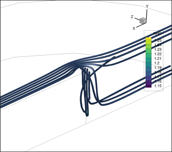
Attributes
Contour group to use for flooding.
The
Indexof theContourGroupto use for flooding.Enable or disable contour flooding display.
Enable lighting effect for streamtrace rod/ribbons.
- StreamtraceRodRibbonContour.flood_contour_group
Contour group to use for flooding.
This property sets and gets the ContourGroup used for flooding. Changing style on this
ContourGroupwill affect all fieldmaps on the sameFramethat use it.Example usage:
>>> group = plot.contour(1) >>> contour = plot.streamtraces.rod_ribbon.contour >>> contour.flood_contour_group = group
- Type:
- StreamtraceRodRibbonContour.flood_contour_group_index
The
Indexof theContourGroupto use for flooding.This property sets and gets, by
Index, theContourGroupused for flooding. Changing style on thisContourGroupwill affect all fieldmaps on the sameFramethat use it.Example usage:
>>> contour = plot.streamtraces.rod_ribbon.contour >>> contour.flood_contour_group_index = 0 # First contour group
- Type:
Index(zero-based index)
- StreamtraceRodRibbonContour.show
Enable or disable contour flooding display.
Example usage:
>>> plot.streamtraces.rod_ribbon.contour.show = True
- Type:
- StreamtraceRodRibbonContour.use_lighting_effect
Enable lighting effect for streamtrace rod/ribbons.
Note
Setting
StreamtraceRodRibbonContour.use_lighting_effectwill also set the same value forStreamtraceRodRibbonShade.use_lighting_effect, and vice-versa.The lighting effect is set with
StreamtraceRodRibbonEffects.lighting_effect, and may be one ofLightingEffect.SmoothWithCreases,LightingEffect.Smooth, orLightingEffect.Paneled.Example usage:
>>> ribbon = plot.streamtraces.rod_ribbon >>> contour = ribbon.contour >>> contour.use_lighting_effect = True >>> ribbon.effects.lighting_effect = LightingEffect.Paneled
- Type:
StreamtraceRodRibbonEffects
- class tecplot.plot.StreamtraceRodRibbonEffects(streamtrace)[source]
Controls how lighting and translucency interacts with streamtrace rods and ribbons.
import os import tecplot from tecplot.constant import * examples_dir = tecplot.session.tecplot_examples_directory() datafile = os.path.join(examples_dir, 'SimpleData', 'DuctFlow.plt') dataset = tecplot.data.load_tecplot(datafile) frame = tecplot.active_frame() frame.plot_type = tecplot.constant.PlotType.Cartesian3D plot = frame.plot() plot.show_mesh = False plot.show_shade = False plot.show_edge = True plot.fieldmap(0).edge.edge_type = EdgeType.Creases plot.show_mesh = False plot.show_shade = False plot.vector.u_variable_index = 3 plot.vector.v_variable_index = 4 plot.vector.w_variable_index = 5 plot.show_streamtraces = True plot.streamtraces.rod_ribbon.width = .03 plot.streamtraces.rod_ribbon.shade.color = Color.Green plot.streamtraces.rod_ribbon.effects.use_translucency = True plot.streamtraces.rod_ribbon.effects.surface_translucency = 80 plot.streamtraces.add_rake(start_position=(1.5, 0, .45), end_position=(1.5, 1, 0), stream_type=Streamtrace.VolumeRibbon) tecplot.export.save_png('streamtrace_ribbon_effects.png', 600, supersample=3)
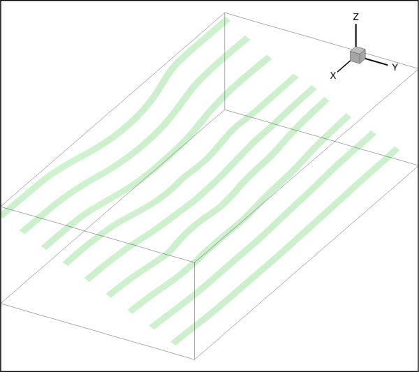
Attributes
Get/set the lighting algorithm used when lighting
Surface translucency of the streamtraces ribbon.
Enable surface translucency.
- StreamtraceRodRibbonEffects.lighting_effect
- Get/set the lighting algorithm used when lighting
streamtrace rods and ribbons.
Ribbon lighting effects must be enabled by setting
StreamtraceRodRibbonShade.use_lighting_effecttoTruewhen setting this value.Note that setting
StreamtraceRodRibbonShade.use_lighting_effectwill also set this value forribbon contours.There are three types of lighting effects: Paneled, SmoothWithCreases and Smooth:
Paneled: Within each cell, the color assigned to each area byshading or contour flooding is tinted by a shade constant across the cell. This shade is based on the orientation of the cell relative to your 3D light source.
SmoothUnlike
Paneledshading that colors the cell surface considering a constant angle to the light relative to the cell’s surface normal,Smoothcomputes the average normal around each cell node and interpolates the lighting influence smoothly across the cell face.SmoothWithCreasesshading is not continuous across zone boundaries unless face neighbors are specified in the data.
SmoothWithCreasesThis option is similar to
Smoothbut considers the crease angle between neighboring, connected cell faces. When the crease angle exceeds the specified amount the edge is considered creased and the lighting interpolation across the cell uses the cell’s surface normal for the shared nodes along that edge instead of the average surface normal at those nodes. If the surface has many edges that exceed the crease angle, such as a very chaotic iso-surface, a significantly larger amount of data is required to render the surface.
Example usage:
>>> plot.streamtraces.rod_ribbon.shade.use_lighting_effect = True >>> plot.streamtraces.rod_ribbon.effects.lighting_effect = LightingEffect.Paneled
- Type:
- StreamtraceRodRibbonEffects.surface_translucency
Surface translucency of the streamtraces ribbon.
Surface translucency must be enabled by setting
StreamtraceRodRibbonEffects.use_translucency=Truewhen setting this value.Valid translucency values range from one (opaque) to 99 (translucent).
Example usage:
>>> plot.streamtraces.rod_ribbon.effects.use_translucency = True >>> plot.streamtraces.rod_ribbon.effects.surface_translucency = 20
- Type:
- StreamtraceRodRibbonEffects.use_translucency
Enable surface translucency.
The surface translucency value can be changed by setting
StreamtraceRodRibbonEffects.surface_translucency.Example usage:
>>> plot.streamtraces.rod_ribbon.effects.use_translucency = True >>> plot.streamtraces.rod_ribbon.effects.surface_translucency = 20
- Type:
StreamtraceRodRibbonMesh
- class tecplot.plot.StreamtraceRodRibbonMesh(robribbon)[source]
Streamtraces rod/ribbon mesh attributes.
Note
To set the mesh color or line thickness, see
Streamtraces.colorandStreamtraces.line_thickness.import os import tecplot from tecplot.constant import * examples_dir = tecplot.session.tecplot_examples_directory() datafile = os.path.join(examples_dir, 'SimpleData', 'DownDraft.plt') dataset = tecplot.data.load_tecplot(datafile) frame = tecplot.active_frame() frame.plot_type = tecplot.constant.PlotType.Cartesian3D plot = frame.plot() plot.fieldmap(0).surfaces.surfaces_to_plot = SurfacesToPlot.BoundaryFaces plot.show_mesh = False plot.show_shade = False plot.show_edge = True plot.vector.u_variable_index = 4 plot.vector.v_variable_index = 5 plot.vector.w_variable_index = 6 plot.show_streamtraces = True ribbon = plot.streamtraces.rod_ribbon ribbon.width = .008 ribbon.mesh.show = True ribbon.mesh.line_thickness = 0.2 #Ribbon mesh color inherited from streamtrace color plot.streamtraces.color = Color.AquaGreen plot.streamtraces.add_rake( start_position=(0, 0.22, 0), end_position=(0, 0.22, 0.1), stream_type=Streamtrace.VolumeRibbon) plot.view.width = 0.644 plot.view.alpha = 66.4 plot.view.theta = -122.4 plot.view.psi = 124.5 plot.view.position = (5.3, 3.56, -4.3) tecplot.export.save_png('streamtrace_ribbon_mesh.png', 600, supersample=3)

Attributes
Get/Set streamtrace rod/ribbon mesh line thickness as a percentage of frame height.
Display mesh.
- StreamtraceRodRibbonMesh.line_thickness
Get/Set streamtrace rod/ribbon mesh line thickness as a percentage of frame height.
Typical values are .02, .1, .4, .8, 1.5
Example usage:
>>> plot.streamtraces.rod_ribbon.mesh.line_thickness = 0.2
- Type:
StreamtraceRodRibbonShade
- class tecplot.plot.StreamtraceRodRibbonShade(streamtrace)[source]
Color and lighting display for rod/ribbons.
import os import tecplot from tecplot.constant import * examples_dir = tecplot.session.tecplot_examples_directory() datafile = os.path.join(examples_dir, 'SimpleData', 'DuctFlow.plt') dataset = tecplot.data.load_tecplot(datafile) frame = tecplot.active_frame() frame.plot_type = tecplot.constant.PlotType.Cartesian3D plot = frame.plot() plot.show_mesh = False plot.show_shade = False plot.show_edge = True plot.fieldmap(0).edge.edge_type = EdgeType.Creases plot.vector.u_variable_index = 3 plot.vector.v_variable_index = 4 plot.vector.w_variable_index = 5 plot.show_streamtraces = True plot.streamtraces.show_paths = True ribbon = plot.streamtraces.rod_ribbon ribbon.shade.show = True ribbon.shade.color = Color.Blue ribbon.shade.use_lighting_effect = True ribbon.width = .03 plot.streamtraces.add_rake(start_position=(1.5, 0, .45), end_position=(1.5, 1, 0), stream_type=Streamtrace.VolumeRibbon) tecplot.export.save_png('streamtrace_ribbon_shade.png', 600, supersample=3)
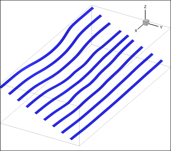
Attributes
Shade color.
Show shade attributes.
Use lighting effect.
- StreamtraceRodRibbonShade.color
Shade color.
Color.MultiColorandColor.RGBColorcoloring are not available. Use flooded contours for multi-color or RGB flooding.Example usage:
>>> plot.streamtraces.rod_ribbon.shade.show = True >>> plot.streamtraces.rod_ribbon.shade.color = Color.Blue
- Type:
- StreamtraceRodRibbonShade.show
Show shade attributes.
Example usage:
>>> plot.streamtraces.rod_ribbon.shade.show = True
- Type:
- StreamtraceRodRibbonShade.use_lighting_effect
Use lighting effect.
When set to
True, the lighting effect may be selected with theSliceEffects.lighting_effectattribute.Note
Setting
SliceShade.use_lighting_effectwill also set the same value forSliceContour.use_lighting_effect, and vice-versa.Example usage:
>>> plot.streamtraces.rod_ribbon.shade.use_lighting_effect = True >>> plot.streamtraces.rod_ribbon.effects.lighting_effect = LightingEffect.Paneled
- Type:
StreamtraceTerminationLine
- class tecplot.plot.StreamtraceTerminationLine(streamtrace)[source]
Streamtraces termination line attributes.
A streamtrace termination line is a polyline that terminates any streamtraces that cross it. The termination line is useful for stopping streamtraces before they spiral or stall.
Note
Before setting any
StreamtraceTerminationLineproperties, you mustadd a termination line.Streamtraces are terminated whenever any of the following occur:
The maximum number of integration steps is reached.
Any point where a streamtrace passes outside the available data.
The streamtrace reaches a point where the velocity magnitude is zero.
import tecplot from tecplot.constant import * import os examples_dir = tecplot.session.tecplot_examples_directory() datafile = os.path.join(examples_dir, 'SimpleData', 'VortexShedding.plt') dataset = tecplot.data.load_tecplot(datafile) frame = tecplot.active_frame() frame.plot_type = tecplot.constant.PlotType.Cartesian2D plot = frame.plot() plot.vector.u_variable = dataset.variable('U(M/S)') plot.vector.v_variable = dataset.variable('V(M/S)') plot.show_streamtraces = True plot.show_shade = True plot.fieldmap(0).shade.color = Color.LightBlue streamtraces = plot.streamtraces streamtraces.set_termination_line([(0.03, 0.005), (0.03, -0.005), ]) term_line = streamtraces.termination_line term_line.active = True term_line.show = True term_line.color = Color.Red term_line.line_pattern = LinePattern.Dashed term_line.pattern_length = .5 term_line.line_thickness = .5 streamtraces.add_rake(start_position=(-0.003, 0.005), end_position=(-0.003, -0.005), stream_type=Streamtrace.TwoDLine, num_seed_points=10) plot.axes.y_axis.min = -0.02 plot.axes.y_axis.max = 0.02 plot.axes.x_axis.min = -0.01 plot.axes.x_axis.max = 0.04 tecplot.export.save_png('streamtrace_term_line.png', 600, supersample=3)
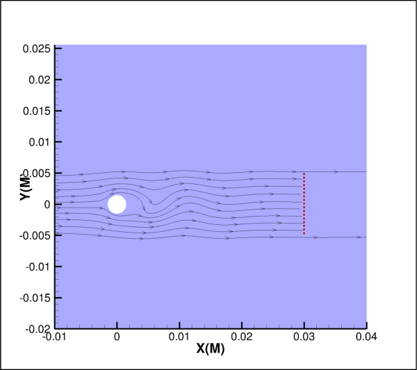
Attributes
Activate/disable the streamtrace termination line.
Color of the termination line.
Pattern of the terminating line.
Thickness of the termination line as a percentage of frame height.
Length of the pattern as a percentage of frame height.
Display the termination line.
- StreamtraceTerminationLine.active
Activate/disable the streamtrace termination line.
Set to
Trueto activate the termination line and terminate any streamtraces that cross it. Set toFalseand redraw the plot with unterminated streamtraces.Example usage:
>>> plot.streamtraces.termination_line.active = True
- Type:
- StreamtraceTerminationLine.color
Color of the termination line.
Example usage:
>>> plot.streamtraces.termination_line.color = Color.Red
- Type:
- StreamtraceTerminationLine.line_pattern
Pattern of the terminating line.
Example usage:
>>> plot.streamtraces.termination_line.line_pattern = LinePattern.Dotted
- Type:
- StreamtraceTerminationLine.line_thickness
Thickness of the termination line as a percentage of frame height.
Example usage:
>>> plot.streamtraces.termination_line.line_thickness = 0.1
- Type:
- StreamtraceTerminationLine.pattern_length
Length of the pattern as a percentage of frame height.
Example usage:
>>> plot.streamtraces.termination_line.pattern_length = 2
- Type:
- StreamtraceTerminationLine.show
Display the termination line.
Set to
Trueto display the termination line. Set toFalseand redraw the plot to display terminated streamlines (ifactiveis set toTrue), but not the termination line itself.Example usage:
>>> plot.streamtraces.termination_line.show = True
- Type:
Text
Font
- class tecplot.text.Font(parent, sv_textshape='TEXTSHAPE')[source]
Style of text objects such as titles and labels.
This class controls the typeface and size of various text objects found in plots and axes:
from os import path import tecplot as tp from tecplot.constant import PlotType, Units, AxisTitleMode examples_dir = tp.session.tecplot_examples_directory() infile = path.join(examples_dir, 'OneraM6wing', 'OneraM6_SU2_RANS.plt') dataset = tp.data.load_tecplot(infile) frame = tp.active_frame() plot = frame.plot(PlotType.Cartesian2D) plot.activate() plot.show_contour = True xaxis = plot.axes.x_axis xaxis.title.title_mode = AxisTitleMode.UseText xaxis.title.text = 'Longitudinal (m)' xaxis.min, xaxis.max = 0, 1.2 yaxis = plot.axes.y_axis yaxis.title.title_mode = AxisTitleMode.UseText yaxis.title.text = 'Transverse (m)' yaxis.min, yaxis.max = 0, 1.3 for ax in [xaxis, yaxis]: ax.title.font.typeface = 'Times' ax.title.font.bold = False ax.title.font.italic = True ax.title.font.size_units = Units.Frame ax.title.font.size = 7 # ensure consistent output between interactive (connected) and batch plot.contour(0).levels.reset_to_nice() tp.export.save_png('font.png', 600, supersample=3)
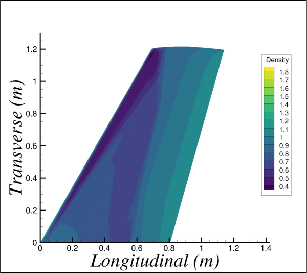
Attributes
Use the bold version of the current typeface.
Use the italic version of the current typeface.
Height of the font.
Used by the size attribute.
Specific font (or typeface) to use for text.
- Font.bold
Use the bold version of the current typeface.
Example:
>>> axis.title.font.bold = True
- Type:
- Font.italic
Use the italic version of the current typeface.
Example:
>>> axis.title.font.italic = True
- Type:
- Font.size
Height of the font. in units of
Font.size_units.Example usage:
>>> axis.title.font.size = 10
- Type:
- Font.size_units
Used by the size attribute.
Possible values:
Units.Point,Units.Frame(percentage of frame height). This example sets the axis title to 10% of the frame height:>>> from tecplot.constant import Units >>> axis.title.font.size_units = Units.Frame >>> axis.title.font.size = 10
- Type:
BaseFont
- class tecplot.text.BaseFont(*svargs, **kwargs)[source]
Plot-level or scatter font style fall-back settings.
Note
Base fonts are accessible directly from line plots (
XYLinePlot.base_font,PolarLinePlot.base_font):>>> frame.plot(PlotType.XYLine).base_font
and the scatter style of field plots (
Scatter.base_font):>>> frame.plot(PlotType.Cartesian3D).scatter.base_font
Attributes
Use the bold version of the current typeface.
Use the italic version of the current typeface.
Specific font (or typeface) to use for text.
- BaseFont.bold
Use the bold version of the current typeface.
Example:
>>> line_plot.base_font.bold = True >>> field_plot.scatter.base_font.bold = True
- Type:
- BaseFont.italic
Use the italic version of the current typeface.
Example:
>>> line_plot.base_font.italic = True >>> field_plot.scatter.base_font.italic = True
- Type:
- BaseFont.typeface
Specific font (or typeface) to use for text.
This can be any font installed on the current system. If the font is not found, Times or Helvetica will be used when rendering the text. Example usage:
>>> line_plot.base_font.typeface = 'Times' >>> field_plot.scatter.base_font.typeface = 'Times'
- Type:
TextBox
- class tecplot.text.TextBox(parent)[source]
Rectangular frame around a text element.
Warning
text.TextBoxobjects cannot be created directly. They are returned by various other read-only properties.Attributes
Type of box surrounding the text.
Color of the box surrounding the text.
Fill color of the box surrounding the text.
Line thickness of the box surrounding the text.
Margin of the box surrounding the text.
- TextBox.box_type
Type of box surrounding the text.
Example usage:
>>> plot = frame.plot() >>> plot.legend.box.box_type = constant.TextBox.None_
- Type:
- TextBox.color
Color of the box surrounding the text.
Example usage:
>>> plot = frame.plot() >>> plot.legend.box.color = Color.Blue
- Type:
- TextBox.fill_color
Fill color of the box surrounding the text.
Example usage:
>>> plot = frame.plot() >>> plot.legend.box.fill_color = Color.Blue
- Type:
- TextBox.line_thickness
Line thickness of the box surrounding the text.
Example usage:
>>> plot = frame.plot() >>> plot.legend.box.line_thickness = 0.2
- Type:
LabelFormat
- class tecplot.text.LabelFormat(labels)[source]
Formatting of numbers shown along in axes and in legends.
This example shows how to format tick label along an axis:
from datetime import datetime import tecplot as tp from tecplot.constant import PlotType, AxisMode, AxisAlignment, NumberFormat tp.new_layout() plot = tp.active_frame().plot(tp.constant.PlotType.Sketch) plot.activate() # setup the plot area margins plot.axes.viewport.left = 10 plot.axes.viewport.right = 90 # show the x-axis, set the title, and alignment with the viewport xaxis = plot.axes.x_axis xaxis.show = True xaxis.title.text = 'Negative numbers in parentheses' xaxis.title.offset = 20 xaxis.line.alignment = AxisAlignment.WithViewport xaxis.line.position = 50 # set limits, tick placement and tick label properties xaxis.ticks.auto_spacing = False xaxis.min, xaxis.max = -5.123e-5, 5.234e-5 xaxis.ticks.spacing = (xaxis.max - xaxis.min) / 6 xaxis.ticks.spacing_anchor = 0 xaxis.tick_labels.angle = 45 xaxis.tick_labels.offset = 3 # format the tick labels in superscript form. example: 1.234x10^5 # format negative numbers to use parentheses instead of a negative sign xformat = xaxis.tick_labels.format xformat.format_type = NumberFormat.SuperScript xformat.precision = 3 xformat.show_negative_sign = False xformat.negative_prefix = '(' xformat.negative_suffix = ')' tp.export.save_png('label_format.png', 600, supersample=3)
Attributes
Index of the custom label to use.
The date/time format to be used.
Type of number formatting to use.
Prefix string to use for negative valued tick labels.
Suffix string to use for negative valued tick labels.
Number of custom label sets available to use.
Prefix string to use for positive valued tick labels.
Suffix string to use for positive valued tick labels.
Number digits after decimal for fixed floating point format.
Strip leading zeros in the formatted number.
Include trailing decimal character with whole numbers.
Include negative sign for negative values.
Prefix string to use for zero valued tick labels.
Suffix string to use for zero valued tick labels.
Methods
add_custom_labels(*labels)Append a list of custom labels as a new set.
custom_labels(index)List of labels for custom labels for set specified by index.
- LabelFormat.add_custom_labels(*labels)[source]
Append a list of custom labels as a new set.
Example usage:
>>> labels = ['apples', 'bananas', 'carrots'] >>> axis.tick_labels.format.add_custom_labels(*labels) >>> print(axis.tick_labels.format.custom_labels(-1)) ['apples', 'bananas', 'carrots']
- LabelFormat.custom_labels(index)[source]
List of labels for custom labels for set specified by index.
Example usage:
>>> axis.tick_labels.format.custom_labels(0) ['apples', 'bananas', 'carrots']
- LabelFormat.custom_labels_index
Index of the custom label to use.
Example usage:
>>> axis.tick_labels.format.custom_labels_index = 0
- Type:
Index(zero-based)
- LabelFormat.datetime_format
The date/time format to be used.
Example usage:
>>> from tecplot.constant import NumberFormat >>> axis.tick_labels.format.format_type = NumberFormat.TimeDate >>> axis.tick_labels.format.datetime_format = 'mmm d, yyyy'
The format can be any combination of the following codes. Placing a backslash in front of a y, m, d, or s in the Time/Date formula will keep it from being processed as part of the formula. All characters not part of the Time/Date formula will appear as entered. For example, “\year yyyy” will appear as “year 2008”, as the backslash keeps the first y from being processed as part of the formula. If you use “m” immediately after the “h” or “hh” code or immediately before the “ss” code, the minutes instead of the month will be displayed.
Years:
yy00-99
yyyy1800-9999
Months:
m1-12
mm01-12
mmmJan-Dec
mmmmJanuary-December
mmmmmfirst letter of the month
Days:
[d]elapsed days
d1-31
dd01-31
dddSun-Sat
ddddSunday-Saturday
dddddS,M,T,W,T,F,S
Hours:
[h]elapsed hours
h0-23 or 1-12
hh00-23 or 1-12
AM/PMAM or PM
A/PAM or PM as “A” or “P”
Minutes:
[m]elapsed minutes
m0-59
mm00-59
Seconds:
s0-59
ss00-59
.0Tenths
.00Hundredths
.000Thousandths
To display the time and date on your plot as a “Sat-Jan-05-2008”, enter the following code:
"ddd-mmm-dd-yyyy"To display the time and date on your plot as a “1-3-08”, enter the following code:
"m-d-yy"To display the time and date on your plot as a “9:30:05 AM”, enter the following code:
"h:mm:ss AM"To display an elapsed time, such as “3:10:15”, enter the following code:
"[d]:hh:mm"- Type:
- LabelFormat.format_type
Type of number formatting to use.
Possible values:
Integer,FixedFloat,Exponential,BestFloat,SuperScript,CustomLabel,LogSuperScript,RangeBestFloat,DynamicLabel,TimeDate.Example usage:
>>> from tecplot.constant import NumberFormat >>> axis.tick_labels.format.format_type = NumberFormat.BestFloat
- Type:
- LabelFormat.negative_prefix
Prefix string to use for negative valued tick labels.
This example shows how to use parentheses instead of a negative sign:
>>> axis.tick_labels.format.show_negative_sign = False >>> axis.tick_labels.format.negative_prefix = '(' >>> axis.tick_labels.format.negative_suffix = ')'
- Type:
- LabelFormat.negative_suffix
Suffix string to use for negative valued tick labels.
This example shows how to use parentheses instead of a negative sign:
>>> axis.tick_labels.format.show_negative_sign = False >>> axis.tick_labels.format.negative_prefix = '(' >>> axis.tick_labels.format.negative_suffix = ')'
- Type:
- LabelFormat.num_custom_labels
Number of custom label sets available to use.
Example usage:
>>> print(axis.tick_labels.format.num_custom_labels) 1
- Type:
- LabelFormat.positive_prefix
Prefix string to use for positive valued tick labels.
Example usage:
>>> axis.tick_labels.format.positive_prefix = 'increase: '
- Type:
- LabelFormat.positive_suffix
Suffix string to use for positive valued tick labels.
Example usage:
>>> axis.tick_labels.format.positive_suffix = ' (m)'
- Type:
- LabelFormat.precision
Number digits after decimal for fixed floating point format.
Example usage:
>>> from tecplot.constant import NumberFormat >>> axis.tick_labels.format.format_type = NumberFormat.FixedFloat >>> axis.tick_labels.format.precision = 3
- Type:
- LabelFormat.remove_leading_zeros
Strip leading zeros in the formatted number.
Example usage:
>>> axis.tick_labels.format.remove_leading_zeros = True
- Type:
- LabelFormat.show_decimals_on_whole_numbers
Include trailing decimal character with whole numbers.
Example usage:
>>> axis.tick_labels.format.show_decimals_on_whole_numbers = True
- Type:
- LabelFormat.show_negative_sign
Include negative sign for negative values.
Example usage:
>>> axis.tick_labels.format.show_negative_sign = True
- Type:
- LabelFormat.zero_prefix
Prefix string to use for zero valued tick labels.
Example usage:
>>> axis.tick_labels.format.zero_prefix = 'origin: '
- Type:
Data Labels
FieldPlotDataLabels
- class tecplot.plot.FieldPlotDataLabels(plot)[source]
Node and cell labels for field plots.
from os import path import tecplot as tp from tecplot.constant import LabelType, NumberFormat, PlotType examples_dir = tp.session.tecplot_examples_directory() infile = path.join(examples_dir, 'SimpleData', 'RainierElevation.plt') dataset = tp.data.load_tecplot(infile) frame = tp.active_frame() plot = frame.plot(PlotType.Cartesian2D) plot.activate() plot.show_contour = True plot.contour(0).legend.show = False plot.axes.x_axis.min = -8500 plot.axes.x_axis.max = 8200 plot.axes.y_axis.min = -400 plot.axes.y_axis.max = -150 plot.data_labels.show_node_labels = True plot.data_labels.node_label_type = LabelType.VarValue plot.data_labels.node_variable = dataset.variable('E') plot.data_labels.index_step = 4 plot.data_labels.label_format.format_type = NumberFormat.Integer plot.data_labels.show_box = False tp.export.save_png('field_plot_data_labels.png')

Attributes
The value to be displayed for cell labels.
Variableto use for cell labels.Indexof the variable to use for cell labels.The
Colorof the data labels.Inherit
Colorfrom the symbol or scatter mapping style.Typeface control for all data labels.
Step interval between labels.
Floating-point number format control.
The value to be displayed for node labels.
Variableto use for node labels.Indexof the variable to use for node labels.Show a box around each label.
Display labels at each cell.
Display labels at each node.
- FieldPlotDataLabels.cell_label_type
The value to be displayed for cell labels.
Possible values are
LabelType.IndexorLabelType.VarValue:>>> plot.data_labels.show_cell_labels = True >>> plot.data_labels.cell_label_type = LabelType.VarValue
- Type:
- FieldPlotDataLabels.cell_variable
Variableto use for cell labels.Example usage:
>>> from tecplot.constant import LabelType >>> plot.data_labels.show_cell_labels = True >>> plot.data_labels.cell_label_type = LabelType.VarValue >>> plot.data_labels.cell_variable = dataset.variable('E')
- Type:
- FieldPlotDataLabels.cell_variable_index
Indexof the variable to use for cell labels.Example usage:
>>> from tecplot.constant import LabelType >>> plot.data_labels.show_cell_labels = True >>> plot.data_labels.cell_label_type = LabelType.VarValue >>> plot.data_labels.cell_variable_index = 3
- Type:
- FieldPlotDataLabels.color
The
Colorof the data labels.Example usage:
>>> from tecplot.constant import Color >>> plot.data_labels.show_node_labels = True >>> plot.data_labels.color = Color.LightBlue
- Type:
- FieldPlotDataLabels.color_by_map
Inherit
Colorfrom the symbol or scatter mapping style.Example usage for linemaps:
>>> from tecplot.constant import Color >>> plot.linemap(0).symbols.color = Color.Blue >>> plot.data_labels.show_node_labels = True >>> plot.data_labels.color_by_map = True
Example usage for fieldmaps:
>>> from tecplot.constant import Color >>> plot.fieldmap(0).scatter.color = Color.Yellow >>> plot.data_labels.show_node_labels = True >>> plot.data_labels.color_by_map = True
- Type:
- FieldPlotDataLabels.font
Typeface control for all data labels.
Example usage:
>>> plot.data_labels.font.typeface = 'Times'
- Type:
- FieldPlotDataLabels.index_step
Step interval between labels.
A value of 1 displays labels on all nodes or cells. Example usage:
>>> plot.data_labels.show_node_labels = True >>> plot.data_labels.index_step = 10
See also
LinePlotDataLabels.step_modefor line plots.- Type:
- FieldPlotDataLabels.label_format
Floating-point number format control.
Example usage:
>>> from tecplot.constant import NumberFormat >>> labels = plot.data_labels >>> labels.label_format.format_type = NumberFormat.Integer
- Type:
- FieldPlotDataLabels.node_label_type
The value to be displayed for node labels.
Possible values are
LabelType.IndexorLabelType.VarValue:>>> from tecplot.constant import LabelType >>> plot.data_labels.show_node_labels = True >>> plot.data_labels.node_label_type = LabelType.VarValue
- Type:
- FieldPlotDataLabels.node_variable
Variableto use for node labels.Example usage:
>>> from tecplot.constant import LabelType >>> plot.data_labels.show_node_labels = True >>> plot.data_labels.node_label_type = LabelType.VarValue >>> plot.data_labels.node_variable = dataset.variable('E')
- Type:
- FieldPlotDataLabels.node_variable_index
Indexof the variable to use for node labels.Example usage:
>>> from tecplot.constant import LabelType >>> plot.data_labels.show_node_labels = True >>> plot.data_labels.node_label_type = LabelType.VarValue >>> plot.data_labels.node_variable_index = 3
- Type:
- FieldPlotDataLabels.show_box
Show a box around each label.
This is
Trueby default. Set toFalseto disable the box:>>> plot.data_labels.show_node_labels = True >>> plot.data_labels.show_box = False
- Type:
- FieldPlotDataLabels.show_cell_labels
Display labels at each cell.
Example usage:
>>> plot.data_labels.show_cell_labels = True
- Type:
LinePlotDataLabels
- class tecplot.plot.LinePlotDataLabels(plot)[source]
Node labels for line plots.
from os import path import tecplot as tp from tecplot.constant import PlotType examples_dir = tp.session.tecplot_examples_directory() infile = path.join(examples_dir, 'SimpleData', 'SunSpots.plt') dataset = tp.data.load_tecplot(infile) frame = tp.active_frame() plot = frame.plot(PlotType.XYLine) plot.activate() plot.data_labels.show_node_labels = True plot.data_labels.index_step = 3 tp.export.save_png('line_plot_data_labels.png')

Attributes
The
Colorof the data labels.Inherit
Colorfrom the symbol or scatter mapping style.Typeface control for all data labels.
Step interval between labels.
Floating-point number format control.
The value to be displayed for node labels.
Show a box around each label.
Display labels at each node.
Distance between labels when stepping by frame units.
The scale to use when stepping through elements.
- LinePlotDataLabels.color
The
Colorof the data labels.Example usage:
>>> from tecplot.constant import Color >>> plot.data_labels.show_node_labels = True >>> plot.data_labels.color = Color.LightBlue
- Type:
- LinePlotDataLabels.color_by_map
Inherit
Colorfrom the symbol or scatter mapping style.Example usage for linemaps:
>>> from tecplot.constant import Color >>> plot.linemap(0).symbols.color = Color.Blue >>> plot.data_labels.show_node_labels = True >>> plot.data_labels.color_by_map = True
Example usage for fieldmaps:
>>> from tecplot.constant import Color >>> plot.fieldmap(0).scatter.color = Color.Yellow >>> plot.data_labels.show_node_labels = True >>> plot.data_labels.color_by_map = True
- Type:
- LinePlotDataLabels.font
Typeface control for all data labels.
Example usage:
>>> plot.data_labels.font.typeface = 'Times'
- Type:
- LinePlotDataLabels.index_step
Step interval between labels.
A value of 1 displays labels on all nodes or cells. Example usage:
>>> plot.data_labels.show_node_labels = True >>> plot.data_labels.index_step = 10
See also
LinePlotDataLabels.step_modefor line plots.- Type:
- LinePlotDataLabels.label_format
Floating-point number format control.
Example usage:
>>> from tecplot.constant import NumberFormat >>> labels = plot.data_labels >>> labels.label_format.format_type = NumberFormat.Integer
- Type:
- LinePlotDataLabels.node_label_type
The value to be displayed for node labels.
Possible values are
LabelType.IndexorLabelType.VarValue:>>> from tecplot.constant import LabelType >>> plot.data_labels.show_node_labels = True >>> plot.data_labels.node_label_type = LabelType.VarValue
- Type:
- LinePlotDataLabels.show_box
Show a box around each label.
This is
Trueby default. Set toFalseto disable the box:>>> plot.data_labels.show_node_labels = True >>> plot.data_labels.show_box = False
- Type:
- LinePlotDataLabels.show_node_labels
Display labels at each node.
Example usage:
>>> plot.data_labels.show_node_labels = True
- Type:
- LinePlotDataLabels.step_distance
Distance between labels when stepping by frame units.
Example usage:
>>> plot.data_labels.show_node_labels = True >>> plot.data_labels.step_mode = StepMode.ByFrameUnits >>> plot.data_labels.step_distance = 10.0
- Type:
- LinePlotDataLabels.step_mode
The scale to use when stepping through elements.
Possible values are:
StepMode.ByIndexandStepMode.ByFrameUnits. Example usage:>>> plot.data_labels.show_node_labels = True >>> plot.data_labels.step_mode = StepMode.ByFrameUnits >>> plot.data_labels.step_distance = 10.0
- Type:
High-Order Element Settings
FieldPlotHOESettings
- class tecplot.plot.FieldPlotHOESettings(frame)[source]
Attributes
Widens or narrows the buffer around sub-element filtering.
Refine element decomposition.
- FieldPlotHOESettings.minmax_scaling_factor
Widens or narrows the buffer around sub-element filtering.
The default value is 1.0. When filtering sub-elements, the extrema (min/max) of an iso-surface or probe variable for the nodes of an sub-element is multiplied by the factor and added as a buffer around the variable min/max range. Example usage:
>>> plot.hoe_settings.minmax_scaling_factor = 4.0
- Type:
- FieldPlotHOESettings.num_subdivision_levels
Refine element decomposition.
With a default setting of 1, the elements are subdivided using only the natural nodes. A value of 2 subdivides elements one level below the natural nodes. Greater than 2 further refines the element decomposition and is more accurate, using the basis functions to compute the manufactured sub-element node values. Each level of subdivisions increases accuracy and time required to render. As a special case, a value of zero is permitted, instructing Tecplot to ignore the high order natural nodes using only the corner nodes for rendering. Example usage:
>>> plot.hoe_settings.num_subdivision_levels = 3
- Type:
Viewport
ReadOnlyViewport
- class tecplot.plot.ReadOnlyViewport(axes)[source]
Attributes
floatin percentage of frame height from the bottom of framefloatin percentage of frame width from the left of the frame.floatin percentage of frame width from the left of the frame.floatin percentage of frame height from the bottom of the frame.
- ReadOnlyViewport.bottom
floatin percentage of frame height from the bottom of frameExample usage:
>>> print(plot.axes.viewport.bottom) 10.0
- ReadOnlyViewport.left
floatin percentage of frame width from the left of the frame.Example usage:
>>> print(plot.axes.viewport.left) 10.0
Viewport
- class tecplot.plot.Viewport(axes)[source]
Attributes
floatin percentage of frame height from the bottom of framefloatin percentage of frame width from the left of the frame.floatin percentage of frame width from the left of the frame.floatin percentage of frame height from the bottom of the frame.
- Viewport.bottom
floatin percentage of frame height from the bottom of frameExample usage:
>>> print(plot.axes.viewport.bottom) 10.0
- Viewport.left
floatin percentage of frame width from the left of the frame.Example usage:
>>> print(plot.axes.viewport.left) 10.0
Cartesian2DViewport
- class tecplot.plot.Cartesian2DViewport(axes)[source]
Attributes
floatin percentage of frame height from the bottom of framefloatin percentage of frame width from the left of the frame.Tolerance for viewport/frame fit niceness.
floatin percentage of frame width from the left of the frame.floatin percentage of frame height from the bottom of the frame.Target value for top when being adjusted or dragged.
Tolerance for snapping to target value for top.
- Cartesian2DViewport.bottom
floatin percentage of frame height from the bottom of frameExample usage:
>>> print(plot.axes.viewport.bottom) 10.0
- Cartesian2DViewport.left
floatin percentage of frame width from the left of the frame.Example usage:
>>> print(plot.axes.viewport.left) 10.0
- Cartesian2DViewport.nice_fit_buffer
Tolerance for viewport/frame fit niceness.
Example usage:
>>> plot.axes.viewport.nice_fit_buffer = 20
- Type:
- Cartesian2DViewport.right
floatin percentage of frame width from the left of the frame.Example usage:
>>> print(plot.axes.viewport.right) 90.0
- Cartesian2DViewport.top
floatin percentage of frame height from the bottom of the frame.Example usage:
>>> print(plot.axes.viewport.top) 90.0
- Cartesian2DViewport.top_snap_target
Target value for top when being adjusted or dragged.
Example usage:
>>> plot.axes.viewport.top_snap_target = 90
- Type:
PolarViewport
- class tecplot.plot.PolarViewport(axes)[source]
Attributes
Border line color around the viewport.
Border line thickness around the viewport.
floatin percentage of frame height from the bottom of frameBackground fill color of the entire viewport.
floatin percentage of frame width from the left of the frame.floatin percentage of frame width from the left of the frame.Draw a border line around the viewport.
floatin percentage of frame height from the bottom of the frame.
- PolarViewport.border_color
Border line color around the viewport.
Example usage:
>>> from tecplot.constant import Color >>> plot.axes.viewport.show_border = True >>> plot.axes.viewport.border_thickness = 0.8 >>> plot.axes.viewport.border_color = Color.Red
- Type:
- PolarViewport.border_thickness
Border line thickness around the viewport.
Example usage:
>>> plot.axes.viewport.show_border = True >>> plot.axes.viewport.border_thickness = 0.8
- Type:
- PolarViewport.bottom
floatin percentage of frame height from the bottom of frameExample usage:
>>> print(plot.axes.viewport.bottom) 10.0
- PolarViewport.fill_color
Background fill color of the entire viewport.
Example usage:
>>> from tecplot.constant import Color >>> plot.axes.viewport.fill_color = Color.Blue
- Type:
- PolarViewport.left
floatin percentage of frame width from the left of the frame.Example usage:
>>> print(plot.axes.viewport.left) 10.0
- PolarViewport.right
floatin percentage of frame width from the left of the frame.Example usage:
>>> print(plot.axes.viewport.right) 90.0
- PolarViewport.show_border
Draw a border line around the viewport.
Example usage:
>>> plot.axes.viewport.show_border = True
- Type:
View and Lighting
Cartesian2DFieldView
- class tecplot.plot.Cartesian2DFieldView(plot, *svargs)[source]
Adjust the way cartesian 2D data is displayed.
from os import path import tecplot as tp from tecplot.constant import PlotType examples_dir = tp.session.tecplot_examples_directory() infile = path.join(examples_dir, 'SimpleData', 'HeatExchanger.plt') dataset = tp.data.load_tecplot(infile) frame = tp.active_frame() plot = frame.plot(PlotType.Cartesian2D) plot.activate() plot.show_contour = True plot.contour(0).variable = dataset.variable('P(N)') plot.contour(0).colormap_name = 'Sequential - Yellow/Green/Blue' plot.view.fit_to_nice() # ensure consistent output between interactive (connected) and batch plot.contour(0).levels.reset_to_nice() tp.export.save_png('view_2D.png', 600, supersample=3)
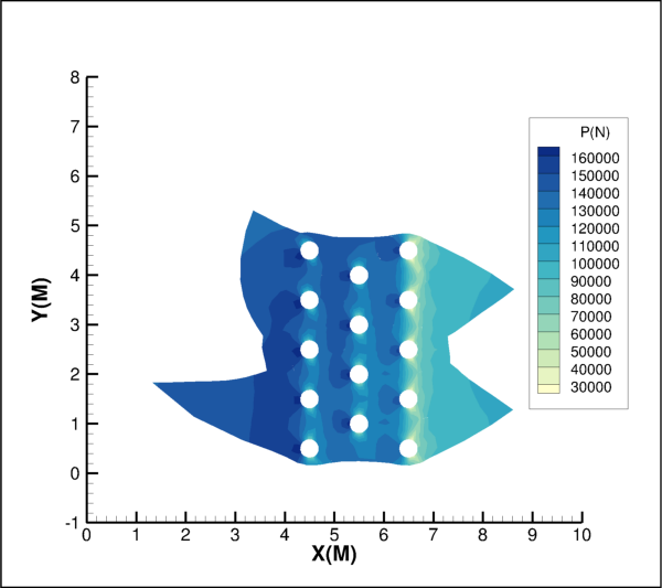
Attributes
Magnification for the data being plotted.
Methods
Shifts axes to make axis-line values "nice"
center([consider_blanking])Center the data within the axis grid area.
fit([consider_blanking])Fit the data being plotted within the axis grid area.
fit_data([consider_blanking])Fit data zones or line mappings within the grid area.
fit_to_nice([consider_blanking])Set axis range to begin/end on major axis increments.
translate([x, y])Shift the data being plotted in the X and/or Y direction.
zoom(xmin, ymin, xmax, ymax)Zoom the view to a rectangular region of the plot.
- Cartesian2DFieldView.adjust_to_nice()
Shifts axes to make axis-line values “nice”
Modifies the axis range to fit the minimum and maximum of the variable assigned to that axis, then snaps the major tick marks to the ends of the axis. If axis dependency is not independent, this may affect the range on another axis.
In other words, given an existing range of values RMin, RMax and an initial delta, D (such as axis ranges with grid spacing or contour levels), determine a new delta (ND) that:
Is 1,2, or 5 times 10 to some power that is the “best” alternative to D.
Produces new range min and max values that are some multiple of ND that are nearest the original RMin and RMax
Axes are shifted without changing the extents of the window.
- Cartesian2DFieldView.center(consider_blanking=True)
Center the data within the axis grid area.
- Cartesian2DFieldView.fit(consider_blanking=True)
Fit the data being plotted within the axis grid area.
Note
This also takes into consideration text and geometries that are plotted using the grid coordinate system.
- Cartesian2DFieldView.fit_data(consider_blanking=True)
Fit data zones or line mappings within the grid area.
- Parameters:
consider_blanking (
Boolean, optional) – IfTrueand blanking is enabled, the resulting view excludes blanked cells at the edges of the plot. If ‘False`, then the resulting view will ignore blanked cells at the edges of the plot. (default:True)
Note
This does not take into consideration text and geometries that are plotted using the grid coordinate system.
- Cartesian2DFieldView.fit_to_nice(consider_blanking=True)[source]
Set axis range to begin/end on major axis increments.
Changes the view to make the extents of the frame neatly hold the plot with integer values for axis labels.
- Cartesian2DFieldView.magnification
Magnification for the data being plotted.
The
magnificationvalue is a decimal percent and must be greater than 0. Amagnificationsize of 1.0 (100%) will size the plot so that it can fit within the grid area. The following example will scale the view to ten percent of the size at which the data would fit the full frame:>>> view.magnification = 0.10
- Type:
- Cartesian2DFieldView.translate(x=0.0, y=0.0)
Shift the data being plotted in the X and/or Y direction.
Note
The amount translated is in frame units.
- Parameters:
x (
float, optional) – Amount to shift in the X direction as a percentage of the frame width. Positive values shift right, negative values shift left. (default: 0.0)y (
float, optional) – Amount to shift in the Y direction as a percentage of the frame height. Positive values shift up, negative values shift down. (default: 0.0)
Translate the view 10 percent of the frame width to the right:
>>> view.translate(x=10)
Translate the view 5 percent of the frame width to the right, 20 of the frame height down:
>>> view.translate(x=5, y=-20)
- Cartesian2DFieldView.zoom(xmin, ymin, xmax, ymax)
Zoom the view to a rectangular region of the plot.
Change the view by “zooming” into the data. Ranges on the axes are adjusted to view the region defined by the rectangle with corners at (
xmin,ymin) and (xmax,ymax).Note
All position values are defined in units of the X- and Y- axis (that is, grid coordinates).
- Parameters:
Zoom so the rectangular region with corners at
(1, 0)and(7, 9)is in view:>>> view.zoom(1, 7, 0, 9)
Cartesian3DView
- class tecplot.plot.Cartesian3DView(plot)[source]
Adjust the way cartesian 3D data is displayed.
import tecplot import os from tecplot.constant import * examples_dir = tecplot.session.tecplot_examples_directory() infile = os.path.join(examples_dir, 'SimpleData', 'F18.plt') ds = tecplot.data.load_tecplot(infile) plot = tecplot.active_frame().plot(PlotType.Cartesian3D) plot.activate() plot.view.width = 17.5 plot.view.alpha = 0 plot.view.theta = 125 plot.view.psi = 65 plot.view.position = (-100, 80, 65) tecplot.export.save_jpeg('view_3D.jpeg', 600, supersample=3)
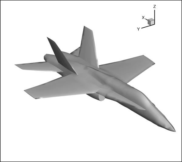
Attributes
Eye origin view Alpha angle in degrees.
Get or set the view distance.
Amount of the plot which is displayed.
Magnification for the data being plotted.
3D viewer position.
Projection type (
PerspectiveorOrthographic).Eye origin view Psi angle in degrees.
Center of rotation for
rotate_axesandrotate_viewer.Eye origin view Theta angle in degrees.
3D view width.
Methods
center([consider_blanking])Center the data within the axis grid area.
fit([consider_blanking])Fit the data being plotted within the axis grid area.
fit_data([consider_blanking])Fit data zones or line mappings within the grid area.
fit_surfaces([consider_blanking])Fit 3D plot surfaces to the grid area.
rotate_axes(angle[, normal])Adjust the view so the axes are rotated about some normal vector.
rotate_to_angles(psi, theta, alpha)Rotate the plot to specific angles.
rotate_viewer(angle[, normal])Rotate the camera or viewer about some normal vector.
translate([x, y])Shift the data being plotted in the X and/or Y direction.
zoom(xmin, ymin, xmax, ymax)Zoom the view to a rectangular region of the plot.
- Cartesian3DView.alpha
Eye origin view Alpha angle in degrees.
The Alpha angle is the twist about the eye origin ray:
>>> plot.view.alpha = 95.0
- Type:
- Cartesian3DView.center(consider_blanking=True)
Center the data within the axis grid area.
- Cartesian3DView.distance
Get or set the view distance.
The view distance is the distance from the viewer to the plane that is parallel to the screen and passes through the 3-D rotation origin.
Note
Changing this value will also change the viewer
position.See also
Example usage:
>>> plot.view.distance 13.5 >>> plot.view.distance = 10.0 >>> plot.view.distance 10.0
- Type:
- Cartesian3DView.field_of_view
Amount of the plot which is displayed.
Get or set the amount of the plot (in terms of spherical arc) in front of the viewer that may be seen.
Warning
field_of_viewcannot be set ifprojectionisProjection.Orthographic.Example usage:
>>> from tecplot.constant import Projection >>> plot.view.projection = Projection.Perspective >>> plot.view.field_of_view = 9.6
- Type:
- Cartesian3DView.fit(consider_blanking=True)
Fit the data being plotted within the axis grid area.
Note
This also takes into consideration text and geometries that are plotted using the grid coordinate system.
- Cartesian3DView.fit_data(consider_blanking=True)
Fit data zones or line mappings within the grid area.
- Parameters:
consider_blanking (
Boolean, optional) – IfTrueand blanking is enabled, the resulting view excludes blanked cells at the edges of the plot. If ‘False`, then the resulting view will ignore blanked cells at the edges of the plot. (default:True)
Note
This does not take into consideration text and geometries that are plotted using the grid coordinate system.
- Cartesian3DView.fit_surfaces(consider_blanking=True)[source]
Fit 3D plot surfaces to the grid area.
- Parameters:
consider_blanking (
bool, optional) – IfTrueand blanking is enabled, the resulting view excludes blanked cells at the edges of the plot. If ‘False`, then the resulting view will ignore blanked cells at the edges of the plot. (default:True)
Note
3D volume zones are excluded when
surfaces_to_plotisSurfacesToPlot.None_.
- Cartesian3DView.magnification
Magnification for the data being plotted.
The
magnificationvalue is a decimal percent and must be greater than 0. Amagnificationsize of 1.0 (100%) will size the plot so that it can fit within the grid area. The following example will scale the view to ten percent of the size at which the data would fit the full frame:>>> view.magnification = 0.10
- Type:
- Cartesian3DView.position
3D viewer position.
The viewer position is the viewer’s relation to the image:
>>> plot.view.position (1.25, 3.2, 0.74) >>> plot.view.position.x 1.25 >>> plot.view.position = (2.5, 0.0, 1.0) >>> plot.view.position.y 0.0 >>> plot.view.position.z 1.0
See also
- Type:
- Cartesian3DView.projection
Projection type (
PerspectiveorOrthographic).When set to
Perspective, Tecplot 360 draws the plot in perspective. When set toOrthographic, the plot is drawn with orthographic projection where the shape of the object does not change with distance.Note
Requires Tecplot version 2017.2 or later.
Example usage:
>>> from tecplot.constant import Projection >>> plot.view.projection = Projection.Orthographic
- Type:
- Cartesian3DView.psi
Eye origin view Psi angle in degrees.
The Psi angle is the tilt of the eye origin ray away from the Z-axis:
>>> plot.view.psi = 90.0
- Type:
- Cartesian3DView.rotate_axes(angle, normal=(0, 0, 1))[source]
Adjust the view so the axes are rotated about some normal vector.
This effectively rotates the axes around the axes origin about some normal using the right-hand rule by the specified angle in degrees. The rotation is performed about the position:
Cartesian3DView.rotation_origin.- Parameters:
Example of rotating 30 degrees about the \(x\)-axis and around the data’s origin:
>>> plot.view.rotation_origin = (0, 0, 0) >>> plot.view.rotate_axes(30, (1, 0, 0))
- Cartesian3DView.rotate_viewer(angle, normal=(0, 0, 1))[source]
Rotate the camera or viewer about some normal vector.
This rotates the viewer about some normal using the right-hand rule by the specified angle in degrees. The rotation is performed about the position:
Cartesian3DView.rotation_origin.- Parameters:
Example of rotating 2 degrees about the \(x\)-axis and around the data’s origin:
>>> plot.view.rotation_origin = (0, 0, 0) >>> plot.view.rotate_viewer(2, (1, 0, 0))
- Cartesian3DView.rotation_origin
Center of rotation for
rotate_axesandrotate_viewer.Example of rotating 30 degrees about the \(y\)-axis and around the data-position \((x, y, z) = (1, 2, 3)\):
>>> plot.view.rotation_origin = (1, 2, 3) >>> plot.view.rotate_axes(30, (0, 1, 0))
- Type:
- Cartesian3DView.theta
Eye origin view Theta angle in degrees.
The Theta angle is the rotation of the eye origin ray about the Z-axis:
>>> plot.view.theta = 24.3
- Type:
- Cartesian3DView.translate(x=0.0, y=0.0)
Shift the data being plotted in the X and/or Y direction.
Note
The amount translated is in frame units.
- Parameters:
x (
float, optional) – Amount to shift in the X direction as a percentage of the frame width. Positive values shift right, negative values shift left. (default: 0.0)y (
float, optional) – Amount to shift in the Y direction as a percentage of the frame height. Positive values shift up, negative values shift down. (default: 0.0)
Translate the view 10 percent of the frame width to the right:
>>> view.translate(x=10)
Translate the view 5 percent of the frame width to the right, 20 of the frame height down:
>>> view.translate(x=5, y=-20)
- Cartesian3DView.width
3D view width.
The 3D view width is the amount of the plot (in X-axis units) in front of the viewer that may be seen.
Warning
widthcannot be set ifprojectionisPerspective.Example usage:
>>> plot.view.width = 1.5
- Type:
- Cartesian3DView.zoom(xmin, ymin, xmax, ymax)
Zoom the view to a rectangular region of the plot.
Change the view by “zooming” into the data. Ranges on the axes are adjusted to view the region defined by the rectangle with corners at (
xmin,ymin) and (xmax,ymax).Note
All position values are defined in units of the X- and Y- axis (that is, grid coordinates).
- Parameters:
Zoom so the rectangular region with corners at
(1, 0)and(7, 9)is in view:>>> view.zoom(1, 7, 0, 9)
XYLineView
- class tecplot.plot.XYLineView(plot)[source]
Adjust the way XY Line data is displayed.
import os import tecplot from tecplot.constant import * examples_dir = tecplot.session.tecplot_examples_directory() datafile = os.path.join(examples_dir, 'SimpleData', 'Rainfall.dat') dataset = tecplot.data.load_tecplot(datafile) frame = tecplot.active_frame() plot = frame.plot() frame.plot_type = tecplot.constant.PlotType.XYLine for i in range(3): plot.linemap(i).show = True plot.linemap(i).line.line_thickness = .4 y_axis = plot.axes.y_axis(0) y_axis.title.title_mode = AxisTitleMode.UseText y_axis.title.text = 'Rainfall (in)' plot.view.fit_to_nice() tecplot.export.save_png('view_line.png', 600, supersample=3)
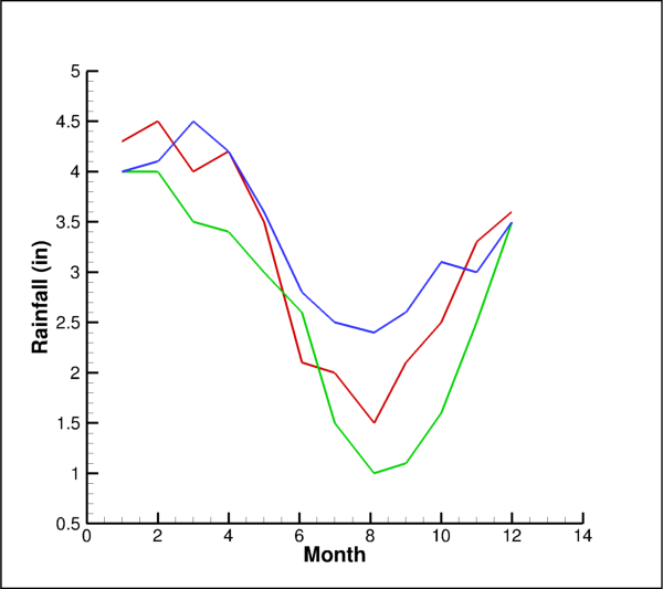
Attributes
Viewport extents in data units.
Magnification for the data being plotted.
Methods
Shifts axes to make axis-line values "nice"
center()Center the data within the axis grid area.
fit()Fit the data being plotted within the axis grid area.
fit_data()Fit data zones or line mappings within the grid area.
Set axis range to begin/end on major axis increments.
translate([x, y])Shift the data being plotted in the X and/or Y direction.
zoom(xmin, ymin, xmax, ymax)Zoom the view to a rectangular region of the plot.
- XYLineView.adjust_to_nice()
Shifts axes to make axis-line values “nice”
Modifies the axis range to fit the minimum and maximum of the variable assigned to that axis, then snaps the major tick marks to the ends of the axis. If axis dependency is not independent, this may affect the range on another axis.
In other words, given an existing range of values RMin, RMax and an initial delta, D (such as axis ranges with grid spacing or contour levels), determine a new delta (ND) that:
Is 1,2, or 5 times 10 to some power that is the “best” alternative to D.
Produces new range min and max values that are some multiple of ND that are nearest the original RMin and RMax
Axes are shifted without changing the extents of the window.
- XYLineView.center()
Center the data within the axis grid area.
- Raises:
TecplotSystemError – View could not be centered.
- XYLineView.extents
Viewport extents in data units.
Extents are represented by the
tuple:(x1, y1, x2, y2)and setting this effectively zooms the view of the data within the viewport. The values(x1, y1)and(x2, y2)are the lower-left and upper-right edges respectively and are in data units. The following example will set the bottom and left edges of the viewport to the value of-3and the top and right edges to the value of 5:>>> plot.view.extents = -3, -3, 5, 5
- Type:
- XYLineView.fit()
Fit the data being plotted within the axis grid area.
Note
This also takes into consideration text and geometries that are plotted using the grid coordinate system.
- XYLineView.fit_data()
Fit data zones or line mappings within the grid area.
Note
This does not take into consideration text and geometries that are plotted using the grid coordinate system.
- XYLineView.fit_to_nice()
Set axis range to begin/end on major axis increments.
Changes the view to make the extents of the frame neatly hold the plot with integer values for axis labels.
- XYLineView.magnification
Magnification for the data being plotted.
The
magnificationvalue is a decimal percent and must be greater than 0. Amagnificationsize of 1.0 (100%) will size the plot so that it can fit within the grid area. The following example will scale the view to ten percent of the size at which the data would fit the full frame:>>> view.magnification = 0.10
- Type:
- XYLineView.translate(x=0.0, y=0.0)
Shift the data being plotted in the X and/or Y direction.
Note
The amount translated is in frame units.
- Parameters:
x (
float, optional) – Amount to shift in the X direction as a percentage of the frame width. Positive values shift right, negative values shift left. (default: 0.0)y (
float, optional) – Amount to shift in the Y direction as a percentage of the frame height. Positive values shift up, negative values shift down. (default: 0.0)
Translate the view 10 percent of the frame width to the right:
>>> view.translate(x=10)
Translate the view 5 percent of the frame width to the right, 20 of the frame height down:
>>> view.translate(x=5, y=-20)
- XYLineView.zoom(xmin, ymin, xmax, ymax)
Zoom the view to a rectangular region of the plot.
Change the view by “zooming” into the data. Ranges on the axes are adjusted to view the region defined by the rectangle with corners at (
xmin,ymin) and (xmax,ymax).Note
All position values are defined in units of the X- and Y- axis (that is, grid coordinates).
- Parameters:
Zoom so the rectangular region with corners at
(1, 0)and(7, 9)is in view:>>> view.zoom(1, 7, 0, 9)
PolarView
- class tecplot.plot.PolarView(plot)[source]
Adjust the way polar data is displayed.
import numpy as np import tecplot as tp from tecplot.constant import PlotType, ThetaMode frame = tp.active_frame() npoints = 300 r = np.linspace(0, 2000, npoints) theta = np.linspace(0, 10, npoints) dataset = frame.create_dataset('Data', ['R', 'Theta']) zone = dataset.add_ordered_zone('Zone', (300,)) zone.values('R')[:] = r zone.values('Theta')[:] = theta plot = frame.plot(PlotType.PolarLine) plot.activate() plot.axes.r_axis.max = np.max(r) plot.axes.theta_axis.mode = ThetaMode.Radians plot.delete_linemaps() lmap = plot.add_linemap('Linemap', zone, dataset.variable('R'), dataset.variable('Theta')) lmap.line.line_thickness = 0.8 plot.view.fit() tp.export.save_png('view_polar.png', 600, supersample=3)
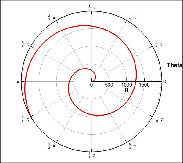
Attributes
Viewport extents in radial data units.
Magnification for the data being plotted.
Methods
center()Center the data within the axis grid area.
fit()Fit the data being plotted within the axis grid area.
fit_data()Fit data zones or line mappings within the grid area.
translate([x, y])Shift the data being plotted in the X and/or Y direction.
zoom(xmin, ymin, xmax, ymax)Zoom the view to a rectangular region of the plot.
- PolarView.center()
Center the data within the axis grid area.
- Raises:
TecplotSystemError – View could not be centered.
- PolarView.extents
Viewport extents in radial data units.
Extents are represented by the
tuple:(x1, y1, x2, y2)and setting this effectively zooms the view of the data within the viewport. The values(x1, y1)and(x2, y2)are the lower-left and upper-right edges respectively and are in radial (data) units. The following example will set the bottom and left edges of the viewport to the radial value of-3and the top and right edges to the radial value of 5:>>> plot.view.extents = -3, -3, 5, 5
- Type:
- PolarView.fit()
Fit the data being plotted within the axis grid area.
Note
This also takes into consideration text and geometries that are plotted using the grid coordinate system.
- PolarView.fit_data()
Fit data zones or line mappings within the grid area.
Note
This does not take into consideration text and geometries that are plotted using the grid coordinate system.
- PolarView.magnification
Magnification for the data being plotted.
The
magnificationvalue is a decimal percent and must be greater than 0. Amagnificationsize of 1.0 (100%) will size the plot so that it can fit within the grid area. The following example will scale the view to ten percent of the size at which the data would fit the full frame:>>> view.magnification = 0.10
- Type:
- PolarView.translate(x=0.0, y=0.0)
Shift the data being plotted in the X and/or Y direction.
Note
The amount translated is in frame units.
- Parameters:
x (
float, optional) – Amount to shift in the X direction as a percentage of the frame width. Positive values shift right, negative values shift left. (default: 0.0)y (
float, optional) – Amount to shift in the Y direction as a percentage of the frame height. Positive values shift up, negative values shift down. (default: 0.0)
Translate the view 10 percent of the frame width to the right:
>>> view.translate(x=10)
Translate the view 5 percent of the frame width to the right, 20 of the frame height down:
>>> view.translate(x=5, y=-20)
- PolarView.zoom(xmin, ymin, xmax, ymax)
Zoom the view to a rectangular region of the plot.
Change the view by “zooming” into the data. Ranges on the axes are adjusted to view the region defined by the rectangle with corners at (
xmin,ymin) and (xmax,ymax).Note
All position values are defined in units of the X- and Y- axis (that is, grid coordinates).
- Parameters:
Zoom so the rectangular region with corners at
(1, 0)and(7, 9)is in view:>>> view.zoom(1, 7, 0, 9)
LightSource
- class tecplot.plot.LightSource(plot)[source]
Three-dimensional light source style control.
The light source is a point of light infinitely far from the drawing area.
from os import path import tecplot as tp from tecplot.constant import PlotType, Color examples_dir = tp.session.tecplot_examples_directory() infile = path.join(examples_dir, 'SimpleData', 'F18.plt') dataset = tp.data.load_tecplot(infile) frame = tp.active_frame() plot = frame.plot(PlotType.Cartesian3D) plot.activate() plot.light_source.direction = (0., -0.7, 0.9) plot.light_source.intensity = 70 plot.light_source.specular_intensity = 80 plot.light_source.specular_shininess = 50 tp.export.save_png('light_source.png')

Attributes
Percentage intensity of the omni-directional fill light.
\((x, y, z)\) direction of the light rays.
Force paneled effects for shaded cell flooding.
Percentage intensity of the light source.
Percentage intensity of specular highlights.
Percentage of shininess for specular highlights.
Percentage of contrast for surface colors.
- LightSource.background_light
Percentage intensity of the omni-directional fill light.
Example usage:
>>> plot.light_source.background_light = 70.0
- Type:
- LightSource.direction
\((x, y, z)\) direction of the light rays.
The direction is in the view coordinate system where \(z\) goes into the page and the origin of \((x, y)\) is in the lower left corner. The default is \((-0.2, -0.2, 0.959)\):
>>> plot.light_source.direction = (0, -0.7, 0.9)
- Type:
- LightSource.force_paneled_for_cell_flood
Force paneled effects for shaded cell flooding.
Example usage:
>>> plot.light_source.force_paneled_for_cell_flood = True
- Type:
- LightSource.intensity
Percentage intensity of the light source.
Example usage:
>>> plot.light_source.intensity = 50.0
- Type:
- LightSource.specular_intensity
Percentage intensity of specular highlights.
Set this to zero to turn off specular effects:
>>> plot.light_source.specular_intensity = 0
- Type:
- LightSource.specular_shininess
Percentage of shininess for specular highlights.
Example usage:
>>> plot.light_source.specular_shininess = 80.0
- Type:
Frame Linking
SketchPlotLinkingBetweenFrames
- class tecplot.plot.SketchPlotLinkingBetweenFrames(frame)[source]
SketchPlotFramestyle linking control.See also
Cartesian3DPlotLinkingBetweenFramesfor details on how to link style across multiple frames.Attributes
Group number (1-32).
Match frame geometry.
Match current solution time.
- SketchPlotLinkingBetweenFrames.group
Group number (1-32).
Each frame may be a member of a single group and may opt in or out of linking each specific style to other frames within this group. Once the group is set, the frame may opt in and out of specific attributes:
>>> frame_linking = plot.linking_between_frames >>> frame_linking.group = 5 >>> frame_linking.link_frame_size_and_position = True >>> frame_linking.link_solution_time = True
- Type:
- SketchPlotLinkingBetweenFrames.link_frame_size_and_position
Match frame geometry.
Keeps the same geometry across all frames in the specified
group. Example usage:>>> frame_linking = plot.linking_between_frames >>> frame_linking.group = 1 >>> frame_linking.link_frame_size_and_position = True
- Type:
Cartesian2DPlotLinkingBetweenFrames
- class tecplot.plot.Cartesian2DPlotLinkingBetweenFrames(frame)[source]
Cartesian2DFieldPlotFramestyle linking control.See also
Cartesian3DPlotLinkingBetweenFramesfor details on how to link style across multiple frames.Attributes
Group number (1-32).
Match axis position within the frames.
Match all contour levels.
Match frame geometry.
Match current solution time.
Match all value blanking style settings.
Match x-axis range.
Match y-axis range.
- Cartesian2DPlotLinkingBetweenFrames.group
Group number (1-32).
Each frame may be a member of a single group and may opt in or out of linking each specific style to other frames within this group. Once the group is set, the frame may opt in and out of specific attributes:
>>> frame_linking = plot.linking_between_frames >>> frame_linking.group = 5 >>> frame_linking.link_frame_size_and_position = True >>> frame_linking.link_solution_time = True
- Type:
- Cartesian2DPlotLinkingBetweenFrames.link_axis_position
Match axis position within the frames.
Keeps the same axis position across all frames in the specified
group. Example usage:>>> frame_linking = plot.linking_between_frames >>> frame_linking.group = 1 >>> frame_linking.link_axis_position = True
- Type:
- Cartesian2DPlotLinkingBetweenFrames.link_contour_levels
Match all contour levels.
Keeps the same contour levels across all frames in the specified
group. Example usage:>>> frame_linking = plot.linking_between_frames >>> frame_linking.group = 1 >>> frame_linking.link_contour_levels = True
- Type:
- Cartesian2DPlotLinkingBetweenFrames.link_frame_size_and_position
Match frame geometry.
Keeps the same geometry across all frames in the specified
group. Example usage:>>> frame_linking = plot.linking_between_frames >>> frame_linking.group = 1 >>> frame_linking.link_frame_size_and_position = True
- Type:
- Cartesian2DPlotLinkingBetweenFrames.link_solution_time
Match current solution time.
Keeps the same active solution time across all frames in the specified
group. Example usage:>>> frame_linking = plot.linking_between_frames >>> frame_linking.group = 1 >>> frame_linking.link_solution_time = True
- Type:
- Cartesian2DPlotLinkingBetweenFrames.link_value_blanking
Match all value blanking style settings.
Keeps the same value blanking across all frames in the specified
group. Example usage:>>> frame_linking = plot.linking_between_frames >>> frame_linking.group = 1 >>> frame_linking.link_value_blanking = True
- Type:
Cartesian3DPlotLinkingBetweenFrames
- class tecplot.plot.Cartesian3DPlotLinkingBetweenFrames(frame)[source]
Cartesian3DFieldPlotFramestyle linking control.The following example shows how to set up a series of transparent overlay frames where each overlay shows one component of the \((U, V, W)\) vector from the
Dataset. All four frames are linked to each other (group 1) so they have the same size, position and view.import os import tecplot as tp from tecplot.constant import * examples_dir = tp.session.tecplot_examples_directory() infile = os.path.join(examples_dir, 'SimpleData', 'DuctFlow.plt') dataset = tp.data.load_tecplot(infile) # Create a "blank" (zeroed-out) variable to use when plotting # only one component of the (U, V, W) vectors tp.data.operate.execute_equation(r'{blank} = 0') # Setup the background frame and plot style frame = tp.active_frame() frame.background_color = Color.Black plot = frame.plot(PlotType.Cartesian3D) plot.activate() contour = plot.contour(0) contour.variable = dataset.variable('P(N/m2)') contour.legend.show = False plot.use_translucency = True plot.show_contour = True plot.show_edge = True plot.axes.orientation_axis.color = Color.White plot.view.width = 2.43 fmap = plot.fieldmap(0) fmap.edge.edge_type = EdgeType.Creases fmap.edge.color = Color.White fmap.surfaces.surfaces_to_plot = SurfacesToPlot.BoundaryFaces frame_linking = plot.linking_between_frames frame_linking.group = 1 frame_linking.link_view = True frame_linking.link_frame_size_and_position = True def add_transparent_overlay(frame): '''Creates a transparent frame overlay with "blank" vector variables.''' overlay_frame = frame.page.add_frame() overlay_frame.transparent = True plot = overlay_frame.plot(frame.plot_type) plot.activate() plot.show_shade = False plot.axes.orientation_axis.show = False blank_var = overlay_frame.dataset.variable('blank') plot.vector.u_variable = blank_var plot.vector.v_variable = blank_var plot.vector.w_variable = blank_var plot.show_vector = True fmap = plot.fieldmap(0) fmap.vector.line_thickness = 0.35 fmap.points.step = 80 fmap.points.points_to_plot = PointsToPlot.AllCellCenters frame_linking = plot.linking_between_frames frame_linking.group = 1 frame_linking.link_view = True frame_linking.link_frame_size_and_position = True return plot # Create three overlays - one for each vector component we want to show u_plot = add_transparent_overlay(frame) u_plot.vector.u_variable = dataset.variable('U(M/S)') u_plot.fieldmap(0).vector.color = Color.Red v_plot = add_transparent_overlay(frame) v_plot.vector.v_variable = dataset.variable('V(M/S)') v_plot.fieldmap(0).vector.color = Color.Green w_plot = add_transparent_overlay(frame) w_plot.vector.w_variable = dataset.variable('W(M/S)') w_plot.fieldmap(0).vector.color = Color.Blue # Now that all plots have been linked, # movement in one will affect all three plots. u_plot.view.translate(x=5) tp.export.save_png('plot3d_linking_between_frames.png')
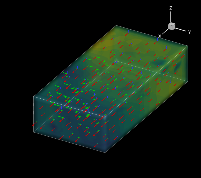
Attributes
Group number (1-32).
Match all contour levels.
Match frame geometry.
Match isosurface values.
Match slice positions.
Match current solution time.
Match all value blanking style settings.
Match the view orientation and position.
- Cartesian3DPlotLinkingBetweenFrames.group
Group number (1-32).
Each frame may be a member of a single group and may opt in or out of linking each specific style to other frames within this group. Once the group is set, the frame may opt in and out of specific attributes:
>>> frame_linking = plot.linking_between_frames >>> frame_linking.group = 5 >>> frame_linking.link_frame_size_and_position = True >>> frame_linking.link_solution_time = True
- Type:
- Cartesian3DPlotLinkingBetweenFrames.link_contour_levels
Match all contour levels.
Keeps the same contour levels across all frames in the specified
group. Example usage:>>> frame_linking = plot.linking_between_frames >>> frame_linking.group = 1 >>> frame_linking.link_contour_levels = True
- Type:
- Cartesian3DPlotLinkingBetweenFrames.link_frame_size_and_position
Match frame geometry.
Keeps the same geometry across all frames in the specified
group. Example usage:>>> frame_linking = plot.linking_between_frames >>> frame_linking.group = 1 >>> frame_linking.link_frame_size_and_position = True
- Type:
- Cartesian3DPlotLinkingBetweenFrames.link_isosurface_values
Match isosurface values.
Keeps the same isosurfaces across all frames in the specified
group. Example usage:>>> frame_linking = plot.linking_between_frames >>> frame_linking.group = 1 >>> frame_linking.link_isosurface_values = True
- Type:
- Cartesian3DPlotLinkingBetweenFrames.link_slice_positions
Match slice positions.
Keeps the same slice positions across all frames in the specified
group. Example usage:>>> frame_linking = plot.linking_between_frames >>> frame_linking.group = 1 >>> frame_linking.link_slice_positions = True
- Type:
- Cartesian3DPlotLinkingBetweenFrames.link_solution_time
Match current solution time.
Keeps the same active solution time across all frames in the specified
group. Example usage:>>> frame_linking = plot.linking_between_frames >>> frame_linking.group = 1 >>> frame_linking.link_solution_time = True
- Type:
- Cartesian3DPlotLinkingBetweenFrames.link_value_blanking
Match all value blanking style settings.
Keeps the same value blanking across all frames in the specified
group. Example usage:>>> frame_linking = plot.linking_between_frames >>> frame_linking.group = 1 >>> frame_linking.link_value_blanking = True
- Type:
XYLinePlotLinkingBetweenFrames
- class tecplot.plot.XYLinePlotLinkingBetweenFrames(frame)[source]
XYLinePlotFramestyle linking control.See also
Cartesian3DPlotLinkingBetweenFramesfor details on how to link style across multiple frames.Attributes
Group number (1-32).
Match axis position within the frames.
Match frame geometry.
Match current solution time.
Match all value blanking style settings.
Match x-axis range.
Match y-axis range.
- XYLinePlotLinkingBetweenFrames.group
Group number (1-32).
Each frame may be a member of a single group and may opt in or out of linking each specific style to other frames within this group. Once the group is set, the frame may opt in and out of specific attributes:
>>> frame_linking = plot.linking_between_frames >>> frame_linking.group = 5 >>> frame_linking.link_frame_size_and_position = True >>> frame_linking.link_solution_time = True
- Type:
- XYLinePlotLinkingBetweenFrames.link_axis_position
Match axis position within the frames.
Keeps the same axis position across all frames in the specified
group. Example usage:>>> frame_linking = plot.linking_between_frames >>> frame_linking.group = 1 >>> frame_linking.link_axis_position = True
- Type:
- XYLinePlotLinkingBetweenFrames.link_frame_size_and_position
Match frame geometry.
Keeps the same geometry across all frames in the specified
group. Example usage:>>> frame_linking = plot.linking_between_frames >>> frame_linking.group = 1 >>> frame_linking.link_frame_size_and_position = True
- Type:
- XYLinePlotLinkingBetweenFrames.link_solution_time
Match current solution time.
Keeps the same active solution time across all frames in the specified
group. Example usage:>>> frame_linking = plot.linking_between_frames >>> frame_linking.group = 1 >>> frame_linking.link_solution_time = True
- Type:
- XYLinePlotLinkingBetweenFrames.link_value_blanking
Match all value blanking style settings.
Keeps the same value blanking across all frames in the specified
group. Example usage:>>> frame_linking = plot.linking_between_frames >>> frame_linking.group = 1 >>> frame_linking.link_value_blanking = True
- Type:
PolarPlotLinkingBetweenFrames
- class tecplot.plot.PolarPlotLinkingBetweenFrames(frame)[source]
PolarLinePlotFramestyle linking control.See also
Cartesian3DPlotLinkingBetweenFramesfor details on how to link style across multiple frames.Attributes
Group number (1-32).
Match frame geometry.
Match current solution time.
Match all value blanking style settings.
Match polar view settings.
- PolarPlotLinkingBetweenFrames.group
Group number (1-32).
Each frame may be a member of a single group and may opt in or out of linking each specific style to other frames within this group. Once the group is set, the frame may opt in and out of specific attributes:
>>> frame_linking = plot.linking_between_frames >>> frame_linking.group = 5 >>> frame_linking.link_frame_size_and_position = True >>> frame_linking.link_solution_time = True
- Type:
- PolarPlotLinkingBetweenFrames.link_frame_size_and_position
Match frame geometry.
Keeps the same geometry across all frames in the specified
group. Example usage:>>> frame_linking = plot.linking_between_frames >>> frame_linking.group = 1 >>> frame_linking.link_frame_size_and_position = True
- Type:
- PolarPlotLinkingBetweenFrames.link_solution_time
Match current solution time.
Keeps the same active solution time across all frames in the specified
group. Example usage:>>> frame_linking = plot.linking_between_frames >>> frame_linking.group = 1 >>> frame_linking.link_solution_time = True
- Type:
- PolarPlotLinkingBetweenFrames.link_value_blanking
Match all value blanking style settings.
Keeps the same value blanking across all frames in the specified
group. Example usage:>>> frame_linking = plot.linking_between_frames >>> frame_linking.group = 1 >>> frame_linking.link_value_blanking = True
- Type: