Data
tecplot.data
Dataset access and manipulation.
A Dataset consists of a matrix of Zones and Variables. Each Zone - Variable pair corresponds to a data
object which can always be treated as a 1D array, but which may be interpreted
as 2D or 3D in the case of ijk-ordered data. In general, the Zone defines the size, shape and connectivity of the data while the
Variable defines the underlying data type and whether the data is nodal or
cell-centered.
Warning
Zero-based Indexing
It is important to know that all indexing in PyTecplot scripts are
zero-based. This is a departure from the macro language which is one-based.
This is to keep with the expectations when working in the python language.
However, PyTecplot does not modify strings that are passed to the
Tecplot Engine. This means that one-based indexing should be used when
running macro commands from python or when using execute_equation().
Loading Data
data.load_tecplot()
- tecplot.data.load_tecplot(filenames, frame=None, read_data_option=ReadDataOption.Append, reset_style=None, initial_plot_first_zone_only=None, initial_plot_type=None, zones=None, variables=None, collapse=None, skip=None, assign_strand_ids=True, add_zones_to_existing_strands=None, include_text=None, include_geom=None, include_custom_labels=None, include_data=None)[source]
Read a tecplot data file.
- Parameters:
filenames (
pathlib.Path,strorlist) – Files to be read. (See note below concerning absolute and relative paths.)frame (
Frame, optional) – TheFrameto attach the resultingDataset. IfNone, the currently activeFrameis used and the zones are appended by default.read_data_option (
ReadDataOption, optional) –Specify how the data is loaded into Tecplot. (default:
ReadDataOption.Append)- Possible values are:
ReadDataOption.ReplaceInActiveFrameThe
Datasetin the active frame is replaced by the newDataset. If other frames were using the sameDatasetoriginally in the active frame, they will continue to use it.
ReadDataOption.AppendAppend to the existing
Dataset.
ReadDataOption.ReplaceReplace the
Datasetattached to the active frame, and to all other frames that use the sameDataset.
Default:
ReadDataOption.Append
reset_style (
bool, optional) – Reset the style for destinationFrame. IfFalse, theFrame’s current style is preserved. (default:True)initial_plot_first_zone_only (
bool, optional) – Informs the Tecplot Engine that after the data is loaded it only needs to activate the first enabled Zone for the initial plot. This option is particularly useful if you have many Zones and want to get the data into the Tecplot Engine and the first Zone drawn as fast as possible. The inactive Zones can always be activated when needed. (default:False)initial_plot_type (
PlotType, optional) – Forces a specific type of plot upon loading of the data. Only used if resetstyle isTrue. To have Tecplot 360 determine the most appropriate plot type for the data, usePlotType.Automatic. Possible values are:PlotType.Automatic(default),Cartesian3D,Cartesian2D,XYLine,PlotType.Sketch,PolarLine.zones (
setofintegers, optional) – Set of Zones to load. UseNoneto load all zones. (default:None)variables (
setofstringsorintegers, optional) – Set ofVariablesto load. If variable names are specified as strings and appending then variables will be aligned with existing variables. If variable offsets are supplied then the variables at those offsets will be loaded and aligned based on the value of the collapse parameter. UseNoneto load all variables. (default:None)collapse (
bool, optional) –Variablesif any are disabled. (default:False)skip – (3-
tupleofintegers, optional) The ijk-skip. A value of (1,1,1) loads every data point in the (i,j,k) directions. A value of (2,2,2) loads every other data point and so forth. This only applies to ordered data. (default: (1,1,1))assign_strand_ids (
bool, optional) – Assign strand ID’s to zones that have a strand ID of -1. (default:True)add_zones_to_existing_strands (
bool, optional) – Add the Zones to matching strands, if they exist. Otherwise, if the new data specifies strands, new ones will be created beginning after the last strand in theDataset. (default:False)include_text (
bool, optional) – Load any text, geometries, or custom labels (default:True)include_geom (
bool, optional) – Load geometries. (default:True)include_data (
bool, optional) – Load data. Set this toFalseif you only want annotations such as text or geometries. (default:True)
- Returns:
- Raises:
TecplotSystemError – Internal error when loading data.
TecplotTypeError – In-valid input.
Note
Absolute and relative paths with PyTecplot
Relative paths, when used within the PyTecplot API are always from Python’s current working directory which can be obtained by calling
os.getcwd(). This is true for batch andconnectedmodes. One exception to this is paths within a macro command or file which will be relative to the Tecplot Engine’s home directory, which is typically the Tecplot 360 installation directory. Finally, when connected to a remote (non-local) instance of Tecplot 360, only absolute paths are allowed.Note that backslashes must be escaped which is especially important for windows paths such as
"C:\\Users"or"\\\\server\\path"which will resolve to"C:\Users"and"\\server\path"respectively. Alternatively, one may use Python’s raw strings:r"C:\Users"andr"\\server\path"
data.load_tecplot_szl()
- tecplot.data.load_tecplot_szl(filenames, frame=None, read_data_option=ReadDataOption.Append, reset_style=None, initial_plot_first_zone_only=None, initial_plot_type=None, assign_strand_ids=True, add_zones_to_existing_strands=None, server=None, connection_method=None, user=None, authentication_method=None, ssh_private_keyfile=PosixPath('~/.ssh/id_rsa'), szlserver_path=None)[source]
Read tecplot SZL data file.
- Parameters:
filenames (
pathlib.Path,strorlist) – Files to be read. (See note below concerning absolute and relative paths.)frame (
Frame, optional) – TheFrameto attach the resultingDataset. IfNone, the currently activeFrameis used and the zones are appended by default.read_data_option (
ReadDataOption, optional) –Specify how the data is loaded into Tecplot. (default:
ReadDataOption.Append)- Possible values are:
ReadDataOption.ReplaceInActiveFrameRemove the dataset from the active frame prior to reading in the new dataset. If other frames use the same
Datasetin the active frame, they will continue to use the old one.
ReadDataOption.AppendAppend to the existing
Dataset. Note also that when appending, the variables in the incoming dataset will be matched up with the existing variables by name and any new variables will be added to the end of the list.
ReadDataOption.ReplaceReplace the
Datasetattached to the active frame and to all other frames that use the sameDataset.
reset_style (
bool, optional) – Reset the style for destinationFrame. IfFalse, theFrame’s current style is preserved. (default:True)initial_plot_first_zone_only (
bool, optional) – Informs the Tecplot Engine that after the data is loaded it only needs to activate the first enabled Zone for the initial plot. This option is particularly useful if you have many Zones and want to get the data into the Tecplot Engine and the first Zone drawn as fast as possible. The inactive Zones can always be activated when needed. (default:False)initial_plot_type (
PlotType, optional) – Forces a specific type of plot upon loading of the data. Only used if resetstyle isTrue. To have Tecplot 360 determine the most appropriate plot type for the data, usePlotType.Automatic. Possible values are:PlotType.Automatic(default),Cartesian3D,Cartesian2D,XYLine,PlotType.Sketch,PolarLine.assign_strand_ids (
bool, optional) – Assign strand ID’s to zones that have a strand ID of -1. (default:True)add_zones_to_existing_strands (
bool, optional) – Add the Zones to matching strands, if they exist. Otherwise, if the new data specifies strands, new ones will be created beginning after the last strand in theDataset. (default:False)server (
str, optional) – Load the data remotely from this server address. When provided, file paths will be relative to the SZL server’s working directory. (default:None)connection_method (
SZLLoader.RemoteConnectionMethod, optional) – When server is given, this specifies the type of connection to be made. Possible values are:SZLLoader.RemoteConnectionMethod.Tunneled(default),SZLLoader.RemoteConnectionMethod.Direct,SZLLoader.RemoteConnectionMethod.Manual.user (
str, optional) – When server is given and connection_method isSZLLoader.RemoteConnectionMethod.TunneledorSZLLoader.RemoteConnectionMethod.Direct, this specifies the username to use when logging into the server. This will default to the client host’s user name.authentication_method (
SZLLoader.RemoteAuthenticationMethod, optional) – The authentication method to use when connecting to the remote server when connection_method isSZLLoader.RemoteConnectionMethod.TunneledorSZLLoader.RemoteConnectionMethod.Direct. Possible values areSZLLoader.RemoteAuthenticationMethod.SSHAgent,SZLLoader.RemoteAuthenticationMethod.SSHPrivateKey(default) which uses the file specified by ssh_private_keyfile orSZLLoader.RemoteAuthenticationMethod.Passwordwhich will prompt the user for the remote login password in the console.ssh_private_keyfile (
pathlib.Pathorstr, optional) – When server is specified and connection_method is set toSZLLoader.RemoteConnectionMethod.TunneledorSZLLoader.RemoteConnectionMethod.Directand when authentication_method is set toSZLLoader.RemoteAuthenticationMethod.SSHPrivateKey, this specifies the full path to the private SSH keyfile. This parameter defaults to~/.ssh/id_rsawhere~expands out to the local user’s home directory.
- Returns:
Note
Absolute and relative paths with PyTecplot
Relative paths, when used within the PyTecplot API are always from Python’s current working directory which can be obtained by calling
os.getcwd(). This is true for batch andconnectedmodes. One exception to this is paths within a macro command or file which will be relative to the Tecplot Engine’s home directory, which is typically the Tecplot 360 installation directory. Finally, when connected to a remote (non-local) instance of Tecplot 360, only absolute paths are allowed.Note that backslashes must be escaped which is especially important for windows paths such as
"C:\\Users"or"\\\\server\\path"which will resolve to"C:\Users"and"\\server\path"respectively. Alternatively, one may use Python’s raw strings:r"C:\Users"andr"\\server\path"
data.load_cfx()
- tecplot.data.load_cfx(filename, frame=None, append=True, assign_strand_ids=True, add_zones_to_existing_strands=True, initial_plot_type=PlotType.Automatic)[source]
Read an ANSYS CFX data file.
- Parameters:
filename (
pathlib.Pathorstr) – The data file to be read. (See note below concerning absolute and relative paths.)frame (
Frame, optional) – TheFrameto attach the resultingDataset. IfNone, the currently activeFrameis used and the zones are appended by default.append (
bool, optional) – Append the data to the existingDataset. IfFalse, the existing data attached to theFrameis deleted and replaced. (default:True)assign_strand_ids (
bool, optional) – Assign strand ID’s to zones that have a strand ID of -1. (default:True)add_zones_to_existing_strands (
bool, optional) – Add the Zones to matching strands, if they exist. Otherwise, if the new data specifies strands, new ones will be created beginning after the last strand in theDataset. (default:True)initial_plot_type (
PlotType, optional) – Set the initial plot type upon loading of the data. Must be one ofPlotType.Automatic(default),PlotType.Cartesian3DorPlotType.Cartesian2D.
- Returns:
Note
Absolute and relative paths with PyTecplot
Relative paths, when used within the PyTecplot API are always from Python’s current working directory which can be obtained by calling
os.getcwd(). This is true for batch andconnectedmodes. One exception to this is paths within a macro command or file which will be relative to the Tecplot Engine’s home directory, which is typically the Tecplot 360 installation directory. Finally, when connected to a remote (non-local) instance of Tecplot 360, only absolute paths are allowed.Note that backslashes must be escaped which is especially important for windows paths such as
"C:\\Users"or"\\\\server\\path"which will resolve to"C:\Users"and"\\server\path"respectively. Alternatively, one may use Python’s raw strings:r"C:\Users"andr"\\server\path"Note
The CFX loader is not available on macOS.
data.load_cgns()
- tecplot.data.load_cgns(filenames, frame=None, read_data_option=ReadDataOption.Append, reset_style=None, initial_plot_first_zone_only=None, initial_plot_type=None, zones=None, variables=None, load_convergence_history=None, combine_fe_sections=None, average_to_nodes='Arithmetic', uniform_grid=None, assign_strand_ids=None, add_zones_to_existing_strands=None, include_boundary_conditions=True)[source]
Read CGNS data files.
- Parameters:
filenames (
pathlib.Path,strorlist) – CGNS data files to be read. (See note below concerning absolute and relative paths.)frame (
Frame, optional) – TheFrameto attach the resultingDataset. IfNone, the currently activeFrameis used and the zones are appended by default.read_data_option (
ReadDataOption, optional) –Specify how the data is loaded into Tecplot. (default:
ReadDataOption.Append)- Possible values are:
ReadDataOption.ReplaceInActiveFrameRemove the dataset from the active frame prior to reading in the new dataset. If other frames use the same
Datasetin the active frame, they will continue to use the old one.
ReadDataOption.AppendAppend to the existing
Dataset.
ReadDataOption.ReplaceReplace the
Datasetattached to the active frame and to all other frames that use the sameDataset.
reset_style (
bool, optional) – Reset the style for destinationFrame. IfFalse, theFrame’s current style is preserved. (default:True)initial_plot_first_zone_only (
bool, optional) – Informs the Tecplot Engine that after the data is loaded it only needs to activate the first enabled Zone for the initial plot. This option is particularly useful if you have many Zones and want to get the data into the Tecplot Engine and the first Zone drawn as fast as possible. The inactive Zones can always be activated when needed. (default:False)initial_plot_type (
PlotType, optional) – Forces a specific type of plot upon loading of the data. Only used if resetstyle isTrue. To have Tecplot 360 determine the most appropriate plot type for the data, usePlotType.Automatic. Possible values are:PlotType.Automatic(default),Cartesian3D,Cartesian2D,XYLine,PlotType.Sketch,PolarLine.zones (
listofintegers, optional) – List of zone indexes to load starting from zero.Noneimplies loading all zones. (default:None)variables (
listofintegers, optional) – List of variable indexes, beyond the first coordinate variables, to load starting from zero.Noneimplies loading all variables. The grid will always be loaded and an index of zero indicates the first non-coordinate variable. (default:None)load_convergence_history (
bool, optional) – Load the global convergence history rather than any grid or solution data. (default:False)combine_fe_sections (
bool, optional) – Combine all finite-element sections with the zone cell-dimension into one zone. (default:False)average_to_nodes (
str, optional) – Average cell-centered data to grid nodes using the specified method. (Options:None, “Arithmetic”, “Laplacian”, default: “Arithmetic”)uniform_grid (
bool, optional) – Indicates the grid structure is the same for all time steps. (default:True)assign_strand_ids (
bool, optional) – Assign strand ID’s to zones that have a strand ID of -1. (default:True)add_zones_to_existing_strands (
bool, optional) – Add the Zones to matching strands, if they exist. Otherwise, if the new data specifies strands, new ones will be created beginning after the last strand in theDataset. (default:False)include_boundary_conditions (
bool, optional) – Load the boundary conditions along with the data. Upon loading, the associated fieldmaps will remain inactive. For unstructured data, boundary conditions are always loaded and this option is ignored. (default:True)
- Returns:
- Raises:
TecplotSystemError – Internal error when loading data.
TecplotTypeError – Invalid input.
Note
Absolute and relative paths with PyTecplot
Relative paths, when used within the PyTecplot API are always from Python’s current working directory which can be obtained by calling
os.getcwd(). This is true for batch andconnectedmodes. One exception to this is paths within a macro command or file which will be relative to the Tecplot Engine’s home directory, which is typically the Tecplot 360 installation directory. Finally, when connected to a remote (non-local) instance of Tecplot 360, only absolute paths are allowed.Note that backslashes must be escaped which is especially important for windows paths such as
"C:\\Users"or"\\\\server\\path"which will resolve to"C:\Users"and"\\server\path"respectively. Alternatively, one may use Python’s raw strings:r"C:\Users"andr"\\server\path"
data.load_converge_cgns()
- tecplot.data.load_converge_cgns(filenames, frame=None, read_data_option=ReadDataOption.Append, reset_style=None)[source]
Read CONVERGE CGNS data files.
- Parameters:
filenames (
pathlib.Path,strorlist) – CONVERGE CGNS data files to be read. (See note below concerning absolute and relative paths.)frame (
Frame, optional) – TheFrameto attach the resultingDataset. IfNone, the currently activeFrameis used and the zones are appended by default.read_data_option (
ReadDataOption, optional) –Specify how the data is loaded into Tecplot. (default:
ReadDataOption.Append)- Possible values are:
ReadDataOption.ReplaceInActiveFrameRemove the dataset from the active frame prior to reading in the new dataset. If other frames use the same
Datasetin the active frame, they will continue to use the old one.
ReadDataOption.AppendAppend to the existing
Dataset.
ReadDataOption.ReplaceReplace the
Datasetattached to the active frame and to all other frames that use the sameDataset.
reset_style (
bool, optional) – Reset the style for destinationFrame. IfFalse, theFrame’s current style is preserved. (default:True)
- Returns:
Note
Absolute and relative paths with PyTecplot
Relative paths, when used within the PyTecplot API are always from Python’s current working directory which can be obtained by calling
os.getcwd(). This is true for batch andconnectedmodes. One exception to this is paths within a macro command or file which will be relative to the Tecplot Engine’s home directory, which is typically the Tecplot 360 installation directory. Finally, when connected to a remote (non-local) instance of Tecplot 360, only absolute paths are allowed.Note that backslashes must be escaped which is especially important for windows paths such as
"C:\\Users"or"\\\\server\\path"which will resolve to"C:\Users"and"\\server\path"respectively. Alternatively, one may use Python’s raw strings:r"C:\Users"andr"\\server\path"
data.load_converge_hdf5()
- tecplot.data.load_converge_hdf5(filenames, frame=None, read_data_option=ReadDataOption.Append, reset_style=None, initial_plot_type=None)[source]
Read CONVERGE HDF5 data files.
- Parameters:
filenames (
pathlib.Path,strorlist) – CONVERGE HDF5 data files to be read. (See note below concerning absolute and relative paths.)frame (
Frame, optional) – TheFrameto attach the resultingDataset. IfNone, the currently activeFrameis used and the zones are appended by default.read_data_option (
ReadDataOption, optional) –Specify how the data is loaded into Tecplot. (default:
ReadDataOption.Append)- Possible values are:
ReadDataOption.ReplaceInActiveFrameRemove the dataset from the active frame prior to reading in the new dataset. If other frames use the same
Datasetin the active frame, they will continue to use the old one.
ReadDataOption.AppendAppend to the existing
Dataset.
ReadDataOption.ReplaceReplace the
Datasetattached to the active frame and to all other frames that use the sameDataset.
reset_style (
bool, optional) – Reset the style for destinationFrame. IfFalse, theFrame’s current style is preserved. (default:True)initial_plot_type (
PlotType, optional) – Forces a specific type of plot upon loading of the data. Only used if resetstyle isTrue. To have Tecplot 360 determine the most appropriate plot type for the data, usePlotType.Automatic. Possible values are:PlotType.Automatic(default),Cartesian3D,Cartesian2D,XYLine,PlotType.Sketch,PolarLine.
- Returns:
Note
Absolute and relative paths with PyTecplot
Relative paths, when used within the PyTecplot API are always from Python’s current working directory which can be obtained by calling
os.getcwd(). This is true for batch andconnectedmodes. One exception to this is paths within a macro command or file which will be relative to the Tecplot Engine’s home directory, which is typically the Tecplot 360 installation directory. Finally, when connected to a remote (non-local) instance of Tecplot 360, only absolute paths are allowed.Note that backslashes must be escaped which is especially important for windows paths such as
"C:\\Users"or"\\\\server\\path"which will resolve to"C:\Users"and"\\server\path"respectively. Alternatively, one may use Python’s raw strings:r"C:\Users"andr"\\server\path"Added in version 2019.1: Loading CONVERGE HDF5 data requires Tecplot 360 2019 R1 or later.
Added in version 1.2.
data.load_converge_output()
- tecplot.data.load_converge_output(filenames, frame=None, read_data_option=ReadDataOption.Append, reset_style=None)[source]
Read CONVERGE Output data files.
- Parameters:
filenames (
pathlib.Path,strorlist) – CONVERGE Output data files to be read. (See note below concerning absolute and relative paths.)frame (
Frame, optional) – TheFrameto attach the resultingDataset. IfNone, the currently activeFrameis used and the zones are appended by default.read_data_option (
ReadDataOption, optional) –Specify how the data is loaded into Tecplot. (default:
ReadDataOption.Append)- Possible values are:
ReadDataOption.ReplaceInActiveFrameRemove the dataset from the active frame prior to reading in the new dataset. If other frames use the same
Datasetin the active frame, they will continue to use the old one.
ReadDataOption.AppendAppend to the existing
Dataset.
ReadDataOption.ReplaceReplace the
Datasetattached to the active frame and to all other frames that use the sameDataset.
reset_style (
bool, optional) – Reset the style for destinationFrame. IfFalse, theFrame’s current style is preserved. (default:True)
- Returns:
Note
Absolute and relative paths with PyTecplot
Relative paths, when used within the PyTecplot API are always from Python’s current working directory which can be obtained by calling
os.getcwd(). This is true for batch andconnectedmodes. One exception to this is paths within a macro command or file which will be relative to the Tecplot Engine’s home directory, which is typically the Tecplot 360 installation directory. Finally, when connected to a remote (non-local) instance of Tecplot 360, only absolute paths are allowed.Note that backslashes must be escaped which is especially important for windows paths such as
"C:\\Users"or"\\\\server\\path"which will resolve to"C:\Users"and"\\server\path"respectively. Alternatively, one may use Python’s raw strings:r"C:\Users"andr"\\server\path"
data.load_ensight()
- tecplot.data.load_ensight(filename, frame=None, read_data_option=ReadDataOption.Append, reset_style=None, initial_plot_first_zone_only=None, initial_plot_type=None, assign_strand_ids=True, add_zones_to_existing_strands=None)[source]
Read Ensight data files and/or boundary file.
- Parameters:
filename (
pathlib.Pathorstr) – The case file to be read. (See note below concerning absolute and relative paths.)frame (
Frame, optional) – TheFrameto attach the resultingDataset. IfNone, the currently activeFrameis used and the zones are appended by default.read_data_option (
ReadDataOption, optional) –Specify how the data is loaded into Tecplot. (default:
ReadDataOption.Append)- Possible values are:
ReadDataOption.ReplaceInActiveFrameRemove the dataset from the active frame prior to reading in the new dataset. If other frames use the same
Datasetin the active frame, they will continue to use the old one.
ReadDataOption.AppendAppend to the existing
Dataset.
ReadDataOption.ReplaceReplace the
Datasetattached to the active frame and to all other frames that use the sameDataset.
reset_style (
bool, optional) – Reset the style for destinationFrame. IfFalse, theFrame’s current style is preserved. (default:True)initial_plot_type (
PlotType, optional) – Forces a specific type of plot upon loading of the data. Only used if resetstyle isTrue. To have Tecplot 360 determine the most appropriate plot type for the data, usePlotType.Automatic. Possible values are:PlotType.Automatic,Cartesian3D,Cartesian2D,XYLine,PlotType.Sketch,PolarLine. (default:PlotType.Automatic)assign_strand_ids (
bool, optional) – Assign strand ID’s to zones that have a strand ID of -1. (default:True)add_zones_to_existing_strands (
bool, optional) – Add the Zones to matching strands, if they exist. Otherwise, if the new data specifies strands, new ones will be created beginning after the last strand in theDataset. (default:True)
- Returns:
Note
Absolute and relative paths with PyTecplot
Relative paths, when used within the PyTecplot API are always from Python’s current working directory which can be obtained by calling
os.getcwd(). This is true for batch andconnectedmodes. One exception to this is paths within a macro command or file which will be relative to the Tecplot Engine’s home directory, which is typically the Tecplot 360 installation directory. Finally, when connected to a remote (non-local) instance of Tecplot 360, only absolute paths are allowed.Note that backslashes must be escaped which is especially important for windows paths such as
"C:\\Users"or"\\\\server\\path"which will resolve to"C:\Users"and"\\server\path"respectively. Alternatively, one may use Python’s raw strings:r"C:\Users"andr"\\server\path"
data.load_fluent()
- tecplot.data.load_fluent(case_filenames=None, data_filenames=None, frame=None, append=True, zones=None, variables=None, all_poly_zones=None, average_to_nodes='Arithmetic', time_interval=None, assign_strand_ids=True, add_zones_to_existing_strands=None, include_particle_data=None, include_additional_quantities=True, save_uncompressed_files=None)[source]
Read Fluent data files.
- Parameters:
case_filenames (
pathlib.Path,strorlist, optional) – Case (.cas, .cas.gz) files to be read. Compressed files with extension .gz are supported. (See note below concerning absolute and relative paths.)data_filenames (
pathlib.Path,strorlist, optional) – Data (.dat, .xml, .dat.gz, .fdat, .fdat.gz, etc.) files to be read. Compressed files with extension .gz are supported.frame (
Frame, optional) – TheFrameto attach the resultingDataset. IfNone, the currently activeFrameis used and the zones are appended by default.append (
bool, optional) – Append the data to the existingDataset. IfFalse, the existing data attached to theFrameis deleted and replaced. (default:True)zones (
strorlistofintegers, optional) – List of zone indexes (zero-based) to load or string specifying the type of zones to load. Possible values are: “CellsAndBoundaries”, “CellsOnly” and “BoundariesOnly”. Specifying one of these options is mutually exclusive with thevariablesoption. (default: “CellsAndBoundaries”)variables (
listofstrings, optional) – List of variable names to load.Noneimplies loading all variables. (default:None)all_poly_zones (
bool, optional) – Converts all zones to Tecplot polytope (polyhedral or polygonal) zones. (default:False)average_to_nodes (
str, optional) – Average cell-centered data to grid nodes using the specified method. (Options:None, “Arithmetic”, “Laplacian”, default: “Arithmetic”)time_interval (
float, optional) – Use a constant time interval between each data (.dat) file. IfNone, the flow-data parameter of each solution data (.dat) file is used. (default:None)assign_strand_ids (
bool, optional) –Assign strand ID’s to zones that have a strand ID of -1. (default:
True)Note
assign_strand_ids only applies if you have also provided a time_interval, otherwise it will be ignored.
add_zones_to_existing_strands (
bool, optional) – Add the Zones to matching strands, if they exist. Otherwise, if the new data specifies strands, new ones will be created beginning after the last strand in theDataset. (default:False)include_particle_data (
bool, optional) – Load particle data from the data (.dat) files. If loading particle data from an XML file, the XML file should be included in thedata_filenameslist. (default:False)include_additional_quantities (
bool, optional) – Load quantities that were derived from the FLUENT’s standard quantities. (default:True) New in Tecplot 360 2017 R2.save_uncompressed_files (
bool, optional) – Save the uncompressed files to the compressed files’ location.
- Returns:
- Raises:
TecplotSystemError – Internal error when loading data.
TecplotTypeError – In-valid input.
Note
Absolute and relative paths with PyTecplot
Relative paths, when used within the PyTecplot API are always from Python’s current working directory which can be obtained by calling
os.getcwd(). This is true for batch andconnectedmodes. One exception to this is paths within a macro command or file which will be relative to the Tecplot Engine’s home directory, which is typically the Tecplot 360 installation directory. Finally, when connected to a remote (non-local) instance of Tecplot 360, only absolute paths are allowed.Note that backslashes must be escaped which is especially important for windows paths such as
"C:\\Users"or"\\\\server\\path"which will resolve to"C:\Users"and"\\server\path"respectively. Alternatively, one may use Python’s raw strings:r"C:\Users"andr"\\server\path"Notes
The
zonesoption takes either alistof zone indexes to be imported or one of “CellsAndBoundaries”, “CellsOnly” or “BoundariesOnly” to indicate the type of zones the user wants to load, however these options are mutually exclusive with thevariablesoption:>>> dataset = tecplot.data.load_fluent(['one.cas', 'two.cas'], ... data_filenames=['one.dat', 'two.dat'], ... variables = ['Pressure','Velocity'], ... zones = [0,1,3])
data.load_fluent_cff()
- tecplot.data.load_fluent_cff(filenames, frame=None, read_data_option=ReadDataOption.Append, reset_style=None, initial_plot_type=None, solution_time_source=None, include_interior_face_zones=None, include_particle_zones=None)[source]
Read Fluent Common Fluids Format files.
- Parameters:
filenames (
pathlib.Path,strorlist) – One or more Fluent CFF case (.cas.h5) files followed by zero or more Fluent CFF data (.dat.h5) files (See note below concerning absolute and relative paths.)frame (
Frame, optional) – TheFrameto attach the resultingDataset. IfNone, the currently activeFrameis used and the zones are appended by default.read_data_option (
ReadDataOption, optional) –Specify how the data is loaded into Tecplot. (default:
ReadDataOption.Append)- Possible values are:
ReadDataOption.ReplaceInActiveFrameRemove the dataset from the active frame prior to reading in the new dataset. If other frames use the same
Datasetin the active frame, they will continue to use the old one.
ReadDataOption.AppendAppend to the existing
Dataset.
ReadDataOption.ReplaceReplace the
Datasetattached to the active frame and to all other frames that use the sameDataset.
reset_style (
bool, optional) – Reset the style for destinationFrame. IfFalse, theFrame’s current style is preserved. (default:True)initial_plot_type (
PlotType, optional) – Forces a specific type of plot upon loading of the data. Only used if resetstyle isTrue. To have Tecplot 360 determine the most appropriate plot type for the data, usePlotType.Automatic. Possible values are:PlotType.Automatic,Cartesian3D,Cartesian2D,XYLine,PlotType.Sketch,PolarLine. (default:PlotType.Automatic)solution_time_source (
FluentCFFLoader.SolutionTimeSource, optional) –Assign the solution times of the zones based on the specified criteria. (default:
FluentCFFLoader.SolutionTimeSource.Auto)- Possible values are:
FluentCFFLoader.SolutionTimeSource.AutoFirst looks for and uses solution time specified in the simulation settings of the Fluent CFF data files. If that information isn’t present in all supplied files, next looks for solution time embedded in
filenames. If solution time cannot be determined, the loader assigns a constant time interval, starting at zero and incrementing by one, if there is a single file, or if there are case and data file combinations, otherwise assigns static solution times of zero.
FluentCFFLoader.SolutionTimeSource.SteadyStateAssigns a static solution time of zero to all zones.
FluentCFFLoader.SolutionTimeSource.ConstantTimeIntervalAssigns a constant time interval, starting at zero and incrementing by one
include_interior_face_zones (
bool, optional) – Interior face zones, which are used to build cell zones, are loaded as independent face zones. (default:False)include_particle_zones (
bool, optional) – Loads particle data as I-ordered zones and nodal variables if it exists in the data (dat.h5) file(s). (default:True)
- Returns:
Note
Absolute and relative paths with PyTecplot
Relative paths, when used within the PyTecplot API are always from Python’s current working directory which can be obtained by calling
os.getcwd(). This is true for batch andconnectedmodes. One exception to this is paths within a macro command or file which will be relative to the Tecplot Engine’s home directory, which is typically the Tecplot 360 installation directory. Finally, when connected to a remote (non-local) instance of Tecplot 360, only absolute paths are allowed.Note that backslashes must be escaped which is especially important for windows paths such as
"C:\\Users"or"\\\\server\\path"which will resolve to"C:\Users"and"\\server\path"respectively. Alternatively, one may use Python’s raw strings:r"C:\Users"andr"\\server\path"Note
The Fluent CFF loader is not available on macOS.
The Fluent CFF loader takes one or more case files, followed by zero or more data files in a single list:
>>> dataset = tecplot.data.load_fluent_cff(
...     ['one.cas.h5', 'one.dat.h5', 'two.dat.h5', 'three.cas.h5'],
...     read_data_option = ReadDataOption.Replace,
...     include_interior_face_zones = True)
Added in version 2021.1: Loading Fluent CFF files requires Tecplot 360 2021 R1 or later.
Added in version 1.4.
data.load_fvcom()
- tecplot.data.load_fvcom(filenames, frame=None, read_data_option=ReadDataOption.Append, reset_style=None, initial_plot_type=None)[source]
Read FVCOM netCDF data files.
- Parameters:
filenames (
pathlib.Path,strorlist) – FVCOM data files to be read. (See note below concerning absolute and relative paths.)frame (
Frame, optional) – TheFrameto attach the resultingDataset. IfNone, the currently activeFrameis used and the zones are appended by default.read_data_option (
ReadDataOption, optional) –Specify how the data is loaded into Tecplot. (default:
ReadDataOption.Append)- Possible values are:
ReadDataOption.ReplaceInActiveFrameRemove the dataset from the active frame prior to reading in the new dataset. If other frames use the same
Datasetin the active frame, they will continue to use the old one.
ReadDataOption.AppendAppend to the existing
Dataset.
ReadDataOption.ReplaceReplace the
Datasetattached to the active frame and to all other frames that use the sameDataset.
reset_style (
bool, optional) – Reset the style for destinationFrame. IfFalse, theFrame’s current style is preserved. (default:True)initial_plot_type (
PlotType, optional) – Forces a specific type of plot upon loading of the data. Only used if resetstyle isTrue. To have Tecplot 360 determine the most appropriate plot type for the data, usePlotType.Automatic. Possible values are:PlotType.Automatic(default),Cartesian3D,Cartesian2D,XYLine,PlotType.Sketch,PolarLine.
- Returns:
Note
Absolute and relative paths with PyTecplot
Relative paths, when used within the PyTecplot API are always from Python’s current working directory which can be obtained by calling
os.getcwd(). This is true for batch andconnectedmodes. One exception to this is paths within a macro command or file which will be relative to the Tecplot Engine’s home directory, which is typically the Tecplot 360 installation directory. Finally, when connected to a remote (non-local) instance of Tecplot 360, only absolute paths are allowed.Note that backslashes must be escaped which is especially important for windows paths such as
"C:\\Users"or"\\\\server\\path"which will resolve to"C:\Users"and"\\server\path"respectively. Alternatively, one may use Python’s raw strings:r"C:\Users"andr"\\server\path"Added in version 2018.2: Loading FVCOM data requires Tecplot 360 2018 R2 or later.
data.load_openfoam()
- tecplot.data.load_openfoam(filename, frame=None, append=True, boundary_zone_construction=None, assign_strand_ids=True, add_zones_to_existing_strands=True, initial_plot_type=PlotType.Automatic, initial_plot_first_zone_only=False)[source]
Read an OpenFOAM data file.
- Parameters:
filename (
pathlib.Pathorstr) – The data file to be read. (See note below concerning absolute and relative paths.)frame (
Frame, optional) – TheFrameto attach the resultingDataset. IfNone, the currently activeFrameis used and the zones are appended by default.append (
bool, optional) – Append the data to the existingDataset. IfFalse, the existing data attached to theFrameis deleted and replaced. (default:True)boundary_zone_construction (
OpenFOAMLoader.BoundaryZoneConstruction, optional) – Set how the boundary zones are constructed. This may be eitherOpenFOAMLoader.BoundaryZoneConstruction.Reconstructed(default) orOpenFOAMLoader.BoundaryZoneConstruction.Decomposed. This option requires Tecplot 360 2019 R1 or later.assign_strand_ids (
bool, optional) – Assign strand ID’s to zones that have a strand ID of -1. (default:True)add_zones_to_existing_strands (
bool, optional) – Add the Zones to matching strands, if they exist. Otherwise, if the new data specifies strands, new ones will be created beginning after the last strand in theDataset. (default:True)initial_plot_type (
PlotType, optional) – Set the initial plot type upon loading of the data. Must be one ofPlotType.Automatic(default),PlotType.Cartesian3DorPlotType.Cartesian2D.initial_plot_first_zone_only (
bool, optional) – Informs the Tecplot Engine that after the data is loaded it only needs to activate the first enabled Zone for the initial plot. This option is particularly useful if you have many Zones and want to get the data into the Tecplot Engine and the first Zone drawn as fast as possible. The inactive Zones can always be activated when needed. (default:False)
- Returns:
Note
Absolute and relative paths with PyTecplot
Relative paths, when used within the PyTecplot API are always from Python’s current working directory which can be obtained by calling
os.getcwd(). This is true for batch andconnectedmodes. One exception to this is paths within a macro command or file which will be relative to the Tecplot Engine’s home directory, which is typically the Tecplot 360 installation directory. Finally, when connected to a remote (non-local) instance of Tecplot 360, only absolute paths are allowed.Note that backslashes must be escaped which is especially important for windows paths such as
"C:\\Users"or"\\\\server\\path"which will resolve to"C:\Users"and"\\server\path"respectively. Alternatively, one may use Python’s raw strings:r"C:\Users"andr"\\server\path"Warning
Zone and variable ordering may change between releases
Due to possible changes in data loaders or data formats over time, the ordering of zones and variables may be different between versions of Tecplot 360. Therefore it is recommended to always reference zones and variables by name instead of by index.
data.load_plot3d()
- tecplot.data.load_plot3d(grid_filenames=None, solution_filenames=None, function_filenames=None, name_filename=None, frame=None, append=True, data_structure=None, is_multi_grid=None, style=None, ascii_is_double=None, ascii_has_blanking=None, uniform_grid=None, assign_strand_ids=True, add_zones_to_existing_strands=True, append_function_variables=None, include_boundaries=True)[source]
Read Plot3D data files.
- Parameters:
grid_filenames (
pathlib.Path,strorlist, optional) – One or more grid file names to be read. (See note below concerning absolute and relative paths.)solution_filenames (
pathlib.Path,strorlist, optional) – One or more solution data file names to be read.function_filenames (
pathlib.Path,strorlist, optional) – One or more function file names.name_filename (
pathlib.Pathorstr, optional) – Path to the name file.frame (
Frame, optional) – TheFrameto attach the resultingDataset. IfNone, the currently activeFrameis used and the zones are appended by default.append (
bool, optional) – Append the data to the existingDataset. IfFalse, the existing data attached to theFrameis deleted and replaced. (default:True)data_structure (
str, optional) – Specifies the data structure and overrides the automatic detection. Options are:1D,2D,3DP,3DW,UNSTRUCTURED. Setting this requiresis_multi_gridandstyleto be set as well.is_multi_grid (
bool, optional) – Sets data as multi-grid and overrides the automatic data structure detection. Setting this requiresdata_structureandstyleto be set as well.style (
bool, optional) – Specifies the data style and overrides the automatic data structure detection. Options are:PLOT3DCLASSIC,PLOT3DFUNCTION,OVERFLOW. Setting this requiresdata_structureandis_multi_gridto be set as well.ascii_is_double (
bool, optional) – Indicates that floating-point numbers found in the text data files should be store with 64-bit precision. (default:False)ascii_has_blanking (
bool, optional) – Indicates that the text data files contain blanking. (default:False)uniform_grid (
bool, optional) – Indicates the grid structure is the same for all time steps. (default:True)assign_strand_ids (
bool, optional) – Assign strand ID’s to zones that have a strand ID of -1. (default:True)add_zones_to_existing_strands (
bool, optional) – Add the Zones to matching strands, if they exist. Otherwise, if the new data specifies strands, new ones will be created beginning after the last strand in theDataset. (default:True)append_function_variables (
bool, optional) – Append variables in function files to those found in solution files. (default:False)include_boundaries (
bool, optional) – Loads boundary zones found in the “.g.fvbnd” file located in the same directory as the grid file, if available. (default:True)
- Returns:
- Raises:
TecplotSystemError – Internal error when loading data.
TecplotValueError – In-valid input.
Note
Absolute and relative paths with PyTecplot
Relative paths, when used within the PyTecplot API are always from Python’s current working directory which can be obtained by calling
os.getcwd(). This is true for batch andconnectedmodes. One exception to this is paths within a macro command or file which will be relative to the Tecplot Engine’s home directory, which is typically the Tecplot 360 installation directory. Finally, when connected to a remote (non-local) instance of Tecplot 360, only absolute paths are allowed.Note that backslashes must be escaped which is especially important for windows paths such as
"C:\\Users"or"\\\\server\\path"which will resolve to"C:\Users"and"\\server\path"respectively. Alternatively, one may use Python’s raw strings:r"C:\Users"andr"\\server\path"Note
Data structure is automatically detected by default.
The options
data_structure,is_multi_gridandstylemust be supplied together or not at all. When all of these areNone, the data structure is automatically detected.The variables from the function files can be appended to the dataset upon loading:
>>> dataset = tecplot.data.load_plot3d(
...     grid_filenames = 'data.g',
...     solution_filenames = ['t0.q', 't1.q'],
...     function_filenames = ['t0.f', 't1.f'],
...     append_function_variables = True)
data.load_telemac()
- tecplot.data.load_telemac(filenames=None, boundary_filename=None, frame=None, read_data_option=ReadDataOption.Append, reset_style=None, initial_plot_type=None)[source]
Read Telemac data files and/or boundary file.
- Parameters:
filenames (
pathlib.Path,strorlist, optional) – Telemac data file(s) to be read. (See note below concerning absolute and relative paths.) Not required if a boundary file is being appended to an existing data set.boundary_filename (
str, optional) – Boundary file. If loaded with multiple Telemac files, will be applied to the first Telemac file. If loaded with no Telemac files, must be appended to an existing data set (read_data_option must beReadDataOption.Append, the default).frame (
Frame, optional) – TheFrameto attach the resultingDataset. IfNone, the currently activeFrameis used and the zones are appended by default.read_data_option (
ReadDataOption, optional) –Specify how the data is loaded into Tecplot. (default:
ReadDataOption.Append)- Possible values are:
ReadDataOption.ReplaceInActiveFrameRemove the dataset from the active frame prior to reading in the new dataset. If other frames use the same
Datasetin the active frame, they will continue to use the old one.
ReadDataOption.AppendAppend to the existing
Dataset.
ReadDataOption.ReplaceReplace the
Datasetattached to the active frame and to all other frames that use the sameDataset.
reset_style (
bool, optional) – Reset the style for destinationFrame. IfFalse, theFrame’s current style is preserved. (default:True)initial_plot_type (
PlotType, optional) – Forces a specific type of plot upon loading of the data. Only used if resetstyle isTrue. To have Tecplot 360 determine the most appropriate plot type for the data, usePlotType.Automatic. Possible values are:PlotType.Automatic,Cartesian3D,Cartesian2D,XYLine,PlotType.Sketch,PolarLine. (default:PlotType.Automatic)
- Returns:
Note
Absolute and relative paths with PyTecplot
Relative paths, when used within the PyTecplot API are always from Python’s current working directory which can be obtained by calling
os.getcwd(). This is true for batch andconnectedmodes. One exception to this is paths within a macro command or file which will be relative to the Tecplot Engine’s home directory, which is typically the Tecplot 360 installation directory. Finally, when connected to a remote (non-local) instance of Tecplot 360, only absolute paths are allowed.Note that backslashes must be escaped which is especially important for windows paths such as
"C:\\Users"or"\\\\server\\path"which will resolve to"C:\Users"and"\\server\path"respectively. Alternatively, one may use Python’s raw strings:r"C:\Users"andr"\\server\path"Added in version 2019.1: Loading Telemac data requires Tecplot 360 2019 R1 or later.
data.load_stl()
- tecplot.data.load_stl(filename, frame=None, append=True, subdivide_zones=SubdivideZones.DoNotSubdivide, assign_strand_ids=True, add_zones_to_existing_strands=True, initial_plot_type=PlotType.Automatic, initial_plot_first_zone_only=False)[source]
Read a 3D Systems STL data file.
- Parameters:
filename (
pathlib.Pathorstr) – The data file to be read. (See note below concerning absolute and relative paths.)frame (
Frame, optional) – TheFrameto attach the resultingDataset. IfNone, the currently activeFrameis used and the zones are appended by default.append (
bool, optional) – Append the data to the existingDataset. IfFalse, the existing data attached to theFrameis deleted and replaced. (default:True)subdivide_zones (
STLLoader.SubdivideZones, optional) – Specify method of zone division. Possible values are:STLLoader.SubdivideZones.DoNotSubdivide(default),STLLoader.SubdivideZones.ByComponentandSTLLoader.SubdivideZones.ByElementType.assign_strand_ids (
bool, optional) – Assign strand ID’s to zones that have a strand ID of -1. (default:True)add_zones_to_existing_strands (
bool, optional) – Add the Zones to matching strands, if they exist. Otherwise, if the new data specifies strands, new ones will be created beginning after the last strand in theDataset. (default:True)initial_plot_type (
PlotType, optional) – Set the initial plot type upon loading of the data. Must be one ofPlotType.Automatic(default),PlotType.Cartesian3DorPlotType.Cartesian2D.initial_plot_first_zone_only (
bool, optional) – Informs the Tecplot Engine that after the data is loaded it only needs to activate the first enabled Zone for the initial plot. This option is particularly useful if you have many Zones and want to get the data into the Tecplot Engine and the first Zone drawn as fast as possible. The inactive Zones can always be activated when needed. (default:False)
- Returns:
Note
Absolute and relative paths with PyTecplot
Relative paths, when used within the PyTecplot API are always from Python’s current working directory which can be obtained by calling
os.getcwd(). This is true for batch andconnectedmodes. One exception to this is paths within a macro command or file which will be relative to the Tecplot Engine’s home directory, which is typically the Tecplot 360 installation directory. Finally, when connected to a remote (non-local) instance of Tecplot 360, only absolute paths are allowed.Note that backslashes must be escaped which is especially important for windows paths such as
"C:\\Users"or"\\\\server\\path"which will resolve to"C:\Users"and"\\server\path"respectively. Alternatively, one may use Python’s raw strings:r"C:\Users"andr"\\server\path"
data.load_vtk()
- tecplot.data.load_vtk(filenames, frame=None, read_data_option=ReadDataOption.Append, reset_style=True, initial_plot_type=PlotType.Automatic, assign_strand_ids=True, add_zones_to_existing_strands=False, solution_time_source=SolutionTimeSource.Auto)[source]
Read VTK data files.
- Parameters:
filenames (
pathlib.Path,strorlist) – The data file(s) to be read. (See note below concerning absolute and relative paths.)frame (
Frame, optional) – TheFrameto attach the resultingDataset. IfNone, the currently activeFrameis used and the zones are appended by default.read_data_option (
ReadDataOption, optional) –Specify how the data is loaded into Tecplot. (default:
ReadDataOption.Append)- Possible values are:
ReadDataOption.ReplaceInActiveFrameThe
Datasetin the active frame is replaced by the newDataset. If other frames were using the sameDatasetoriginally in the active frame, they will continue to use it.
ReadDataOption.AppendAppend to the existing
Dataset.
ReadDataOption.ReplaceReplace the
Datasetattached to the active frame, and to all other frames that use the sameDataset.
Default:
ReadDataOption.Append
reset_style (
bool, optional) – Reset the style for destinationFrame. IfFalse, theFrame’s current style is preserved. (default:True)initial_plot_type (
PlotType, optional) – Forces a specific type of plot upon loading of the data. Only used if resetstyle isTrue. To have Tecplot 360 determine the most appropriate plot type for the data, usePlotType.Automatic. Possible values are:PlotType.Automatic(default),Cartesian3D,Cartesian2D,XYLine,PlotType.Sketch,PolarLine.assign_strand_ids (
bool, optional) – Assign strand ID’s to zones that have a strand ID of -1. (default:True)add_zones_to_existing_strands (
bool, optional) – Add the Zones to matching strands, if they exist. Otherwise, if the new data specifies strands, new ones will be created beginning after the last strand in theDataset. (default:False)solution_time_source (
VTKLoader.SolutionTimeSource, optional) – Assign the solution times of the zones based on the specified criteria. Possible values are:VTKLoader.SolutionTimeSource.Auto(default) which favors the “time” scalar over the numbers embedded in the file names,VTKLoader.SolutionTimeSource.None_which does not assign solutions times or strands,VTKLoader.SolutionTimeSource.FromFieldDatawhich uses the “time” scalar andVTKLoader.SolutionTimeSource.FromFilenamewhich uses the solution time embedded in the file names.
- Returns:
Note
Absolute and relative paths with PyTecplot
Relative paths, when used within the PyTecplot API are always from Python’s current working directory which can be obtained by calling
os.getcwd(). This is true for batch andconnectedmodes. One exception to this is paths within a macro command or file which will be relative to the Tecplot Engine’s home directory, which is typically the Tecplot 360 installation directory. Finally, when connected to a remote (non-local) instance of Tecplot 360, only absolute paths are allowed.Note that backslashes must be escaped which is especially important for windows paths such as
"C:\\Users"or"\\\\server\\path"which will resolve to"C:\Users"and"\\server\path"respectively. Alternatively, one may use Python’s raw strings:r"C:\Users"andr"\\server\path"
Saving Data
data.save_tecplot_ascii()
- tecplot.data.save_tecplot_ascii(filename, frame=None, dataset=None, zones=None, variables=None, include_text=None, precision=None, include_geom=None, include_data=None, include_data_share_linkage=None, include_autogen_face_neighbors=None, use_point_format=None, include_custom_labels=None)[source]
Write Tecplot ASCII data file.
- Parameters:
filename (
pathlib.Pathorstr) – Name of the data file to write. (See note below conerning absolute and relative paths.)frame (
Frame, optional) – TheFramewhich holds theDatasetto be written. If this option and dataset are bothNone, the currently activeFrameis used. (default:None)dataset (
Dataset, optional) – TheDatasetto write out. If this and frame are bothNone, theDatasetof the currently activeFrameis used. (default:None)include_text (
bool, optional) – Write out all text (default:True)include_geom (
bool, optional) – Write out all geometries. (default:True)include_data (
bool, optional) – Write out the data. Set this toFalseif you only want to write out annotations. (default:True)include_data_share_linkage (
bool, optional) – Conserve space and write the variable and connectivity linkage wherever possible. IfFalse, this will write out all data, losing the connectivity sharing linkage for future dataset reads of the file. (default:False)include_autogen_face_neighbors (
bool, optional) – Save the face neighbor connectivity. This may produce very large data files. (default:False)include_custom_labels (
bool, optional) – Write out any custom labels in the dataset to the output data file. (default:True)use_point_format (
bool, optional) – Write out point format, otherwise use block format. (default:False)zones (
listof Zones, optional) – Zones to write out. UseNoneto write out all Zones. (default:None)variables (
listofVariables, optional) –Variablesto write out. UseNoneto write out allVariables. (default:None)precision (
int, optional) – ASCII decimal precision to use. (default: 12)
- Returns:
- Raises:
Note
Absolute and relative paths with PyTecplot
Relative paths, when used within the PyTecplot API are always from Python’s current working directory which can be obtained by calling
os.getcwd(). This is true for batch andconnectedmodes. One exception to this is paths within a macro command or file which will be relative to the Tecplot Engine’s home directory, which is typically the Tecplot 360 installation directory. Finally, when connected to a remote (non-local) instance of Tecplot 360, only absolute paths are allowed.Note that backslashes must be escaped which is especially important for windows paths such as
"C:\\Users"or"\\\\server\\path"which will resolve to"C:\Users"and"\\server\path"respectively. Alternatively, one may use Python’s raw strings:r"C:\Users"andr"\\server\path"Example
In this example, we load sample data and save the data in Tecplot ASCII format:
from os import path
import tecplot
examples_directory = tecplot.session.tecplot_examples_directory()
infile = path.join(examples_directory,
                   'OneraM6wing', 'OneraM6_SU2_RANS.plt')
dataset = tecplot.data.load_tecplot(infile)
variables_to_save = [dataset.variable(V)
                     for V in ('x','y','z','Pressure_Coefficient')]

zone_to_save = dataset.zone('WingSurface')
# write data out to an ascii file
tecplot.data.save_tecplot_ascii('wing.dat', dataset=dataset,
                                variables=variables_to_save,
                                zones=[zone_to_save])
data.save_tecplot_plt()
- tecplot.data.save_tecplot_plt(filename, frame=None, dataset=None, zones=None, variables=None, version=None, include_text=None, include_geom=None, include_data=None, include_data_share_linkage=None, include_autogen_face_neighbors=None, associate_with_layout=None, include_custom_labels=None)[source]
Write Tecplot binary PLT data file.
- Parameters:
filename (
pathlib.Pathorstr) – Name of the data file to write. (See note below conerning absolute and relative paths.)frame (
Frame, optional) – TheFramewhich holds theDatasetto be written. If this option and dataset are bothNone, the currently activeFrameis used. (default:None)dataset (
Dataset, optional) – TheDatasetto write out. If this and frame are bothNone, theDatasetof the currently activeFrameis used. (default:None)zones (
listof Zones, optional) – Zones to write out. IfNone, all Zones will be saved.variables (
listofVariables, optional) –Variablesto write out. IfNone, allVariableswill be saved.include_text (
bool, optional) – Write out all text. (default:True)include_geom (
bool, optional) – Write out all geometries. (default:True)include_data (
bool, optional) – Write out the data. Set this toFalseif you only want to write out annotations. (default:True)include_data_share_linkage (
bool, optional) – Conserve space and write the variable and connectivity linkage wherever possible. IfFalse, this will write out all data, losing the connectivity sharing linkage for future dataset reads of the file. (default:False)include_autogen_face_neighbors (
bool, optional) – Save the face neighbor connectivity. This may produce very large data files. (default:False)include_custom_labels (
bool, optional) – Write out any custom labels in the dataset to the output data file. (default:True)associate_with_layout (
bool, optional) – Associate this data file with the current layout. Set toFalseto write the datafile without modifying Tecplot’s current data file to layout association. If version is set to anything other thanBinaryFileVersion.Current, this association is not possible, and this parameter will be ignored. (default:True)version (
BinaryFileVersion, optional) – Specifies the file version to write. Note that some data may be excluded from the file if it cannot be supported in the specified version. Possible values are:Tecplot2006,Tecplot2008,Tecplot2009andBinaryFileVersion.Current. (default:BinaryFileVersion.Current)
- Returns:
- Raises:
Note
Absolute and relative paths with PyTecplot
Relative paths, when used within the PyTecplot API are always from Python’s current working directory which can be obtained by calling
os.getcwd(). This is true for batch andconnectedmodes. One exception to this is paths within a macro command or file which will be relative to the Tecplot Engine’s home directory, which is typically the Tecplot 360 installation directory. Finally, when connected to a remote (non-local) instance of Tecplot 360, only absolute paths are allowed.Note that backslashes must be escaped which is especially important for windows paths such as
"C:\\Users"or"\\\\server\\path"which will resolve to"C:\Users"and"\\server\path"respectively. Alternatively, one may use Python’s raw strings:r"C:\Users"andr"\\server\path"Example
In this example, we load sample data and save the data in Tecplot binary PLT format:
from os import path
import tecplot
examples_directory = tecplot.session.tecplot_examples_directory()
infile = path.join(examples_directory,
                   'OneraM6wing', 'OneraM6_SU2_RANS.plt')
dataset = tecplot.data.load_tecplot(infile)
variables_to_save = [dataset.variable(V)
                     for V in ('x', 'y', 'z',
                               'Pressure_Coefficient')]

zone_to_save = dataset.zone('WingSurface')
# write data out to a binary file
tecplot.data.save_tecplot_plt('wing.plt', dataset=dataset,
                                variables=variables_to_save,
                                zones=[zone_to_save])
data.save_tecplot_szl()
- tecplot.data.save_tecplot_szl(filename, frame=None, dataset=None)[source]
Write Tecplot SZL data file.
- Parameters:
filename (
pathlib.Pathorstr) – Name of the data file to write. (See note below conerning absolute and relative paths.)frame (
Frame, optional) – TheFramewhich holds theDatasetto be written. If this option and dataset are bothNone, the currently activeFrameis used. (default:None)dataset (
Dataset, optional) – TheDatasetto write out. If this and frame are bothNone, theDatasetof the currently activeFrameis used. (default:None)
- Returns:
Note
Absolute and relative paths with PyTecplot
Relative paths, when used within the PyTecplot API are always from Python’s current working directory which can be obtained by calling
os.getcwd(). This is true for batch andconnectedmodes. One exception to this is paths within a macro command or file which will be relative to the Tecplot Engine’s home directory, which is typically the Tecplot 360 installation directory. Finally, when connected to a remote (non-local) instance of Tecplot 360, only absolute paths are allowed.Note that backslashes must be escaped which is especially important for windows paths such as
"C:\\Users"or"\\\\server\\path"which will resolve to"C:\Users"and"\\server\path"respectively. Alternatively, one may use Python’s raw strings:r"C:\Users"andr"\\server\path"Example
In this example, we load sample data and save it in Tecplot SZL format:
from os import path
import tecplot
examples_directory = tecplot.session.tecplot_examples_directory()
infile = path.join(examples_directory,
                   'OneraM6wing', 'OneraM6_SU2_RANS.plt')
dataset = tecplot.data.load_tecplot(infile)
tecplot.data.save_tecplot_szl('wing.szplt')
Data Queries
data.query.probe_at_position()
- tecplot.data.query.probe_at_position(x, y, z=None, nearest=False, starting_cell=None, starting_zone=None, zones=None, dataset=None, frame=None)[source]
Returns field values at a point in space.
Note
The position is taken according to the axis assignments of the
Framewhich may be any of the associated variables in theDatasetand not necessarily(X, Y, Z). See:Cartesian3DFieldAxis.variable.- Parameters:
x (
float, z is optional) – position to probe for field values.y (
float, z is optional) – position to probe for field values.z (
float, z is optional) – position to probe for field values.nearest (
bool) – Returns the values at the nearest node to the given position. Probe position must be inside the volume of the data being queried, otherwise this will returnNone.starting_cell (3-
tupleofintegers, optional) – The(i,j,k)-index of the cell to start looking for the given position. This must be used withstarting_zone.starting_zone (Zone, optional) – The first zone to start searching. This is required only when
starting_cellis specified.zones (
listof Zones, optional) – Limits the search to the given zones.Noneimplies searching all zones. (default:None)dataset (
Dataset, optional) – TheDatasetto probe. (defaults to the activeDataset.)frame (
Frame, optional) – TheFramewhich determines the spatial variable assignment(X,Y,Z). (defaults to the activeFrame.)
- Returns:
-
(data, cell, zone):
Note
Returns
Noneif the position can’t be probed.This method will return
Noneif the position is outside the volume of the data being queried. This means one should capture the results in a single variable and test it againstNonebefore proceeding:result = tp.data.query.probe_at_position(1.0, 2.0, 3.0) if result is None: print('probe failed.') else: data, cell, zone = result
Additionally, with Tecplot 360 versions 2018 R1 and later, this function will raise an exception if Tecplot 360 was interrupted via the GUI during the probe operation.
data.query.probe_on_surface()
- tecplot.data.query.probe_on_surface(positions=((0,), (0,), (0,)), zones=None, variables=None, probe_nearest=ProbeNearest.Position, obey_blanking=True, num_nearest_nodes=20, tolerance=1e-05, dataset=None, frame=None)[source]
Returns field values at points on a surface closest the points given.
Note
The positions are processed according to the axis assignments of the
Framewhich may be any of the associated variables in theDatasetand not necessarily (but usually)(X, Y, Z). See:Cartesian3DFieldAxis.variable.- Parameters:
positions (2D
floatarray) – Array of points to probe dimensioned by(3, N)where the first dimension corresponds to(x, y, z). A 1Dfloatarray is accepted for single point probes, however this should be avoided when probing several positions as the internal algorithm is optimized for probing many positions at once.zones (
listof Zones, optional) – Limits the search to the given zones.Noneimplies searching all active relevant surface zones including surfaces of ordered volume zones. To search FE or polygonal volume boundaries, include the volume zones in this list. (default:None)variables (
listofVariables, optional) – The variables within the dataset to probe.Noneimplies all variables. (default:None)probe_nearest (
ProbeNearest, optional) – Probe at the nodal location (ProbeNearest.Node) or interpolate to nearest location on the surface (ProbeNearest.Position, default). The return parameter cells_or_nodes will be cells if set toProbeNearest.Position(default), or nodes if set toProbeNearest.Node.obey_blanking (
bool, optional) – Do not search blanked cells according the frame’s style settings. (default:True)num_nearest_nodes (
int, optional) – Only consider surface cells that contain one of the closestNnodes to the probed position. For highly varying surfaces, the nearest cell may or may not contain the nearest nodes to the probe position and so this value should be increased accordingly, however doing so increases the search-space linearly. (default: 20)tolerance (
float, optional) – The percentage of the longest cartesian(x, y, z)dimension subtended by the polygons of the surface. This is used in several parts of the algorithm to find the nearest position on the surface zones and should be increased when probing imprecise nodal position data. (default: 1e-5)dataset (
Dataset, optional) – TheDatasetto probe. (defaults to the activeDataset.)frame (
Frame, optional) – TheFramewhich determines the spatial variable assignment(X,Y,Z). (defaults to the activeFrame.)
- Returns:
namedtuple–(data, cells_or_nodes, planes, zone):data(listoffloats)Flattened
floatarray which can be reshaped to(V, N)whereVis the number of variables returned (either the number of variables in the dataset or the length of variables input parameter) andNis the number of points probed.cells_or_nodes(listofintegers)The index to the cells (or nodes if
ProbeNearest.Nodewas passed in to probe_nearest) containing the returned positions.planes(listofIJKPlanes)For ordered zones, these are the plane-orientations of the cells for each probed position.
zones(listof Zones)Zones containing the given positions.
Added in version 2018.1: Probe on surface requires Tecplot 360 2018 R1 or later.
Note
The frame’s plot type must be set to
PlotType.Cartesian3DProbe on surface requires the spatial variables to be set according to the frame’s style. This can be done by setting the plot type to
PlotType.Cartesian3D. Example:tp.active_frame().plot_type = tp.constant.PlotType.Cartesian3D
For probing on 2D data, use
probe_at_position().Note
Linear zones will always return nearest nodal values.
If linear zones, which are ignored by default, are included in the zones parameter, the resulting values on that zone will always be nodal and no interpolation on the position will be done.
Note
Irregular or jaggged surfaces may behave poorly.
For performance reasons, this algorithm has the potential to miss the closest position on highly varying surfaces. This can be addressed by first increasing num_nearest_nodes to search more of the zones and then by increasing the tolerance to allow for imprecise position data - skewed polygons for example.
All nodes of each cell considered are checked for co-planarity. This check can be relaxed slightly by increasing the tolerance parameter. The nearest position calculation will then be made assuming the cells are planar and the resulting positions may be imprecise.
Example usage:
from os import path
import numpy as np

import tecplot as tp
from tecplot.constant import PlotType

examples = tp.session.tecplot_examples_directory()
datafile = path.join(examples, 'SimpleData', 'F18.plt')
ds = tp.data.load_tecplot(datafile)
fr = tp.active_frame()
fr.plot_type = PlotType.Cartesian3D

# probe a single point
res = tp.data.query.probe_on_surface((13.5, 4.0, 0.6 ))

'''
The following line will print:
    (13.499723788684996, 3.9922783797612795, 0.49241572276992346,
    0.0018958827755862578, 0.07313805429221854, 0.997276718375976,
    0.06335166319722907)
'''
print(res.data)

# probe multiple points
points = np.array([[13.5,  4.0, 0.6],  # just above starboard wing
                   [13.5, -4.0, 0.6]]) # just above port wing

res = tp.data.query.probe_on_surface(points.transpose())
values = np.array(res.data).reshape((-1, len(points))).transpose()

'''
The following will print the probed position and the result of the probe
    [ 13.5   4.    0.6] [  1.34997238e+01   3.99227838e+00   4.92415723e-01
       1.89588278e-03   7.31380543e-02   9.97276718e-01   6.33516632e-02]
    [ 13.5  -4.    0.6] [  1.34997238e+01  -3.99227838e+00   4.92415723e-01
       1.89588278e-03   7.31380543e-02   9.97276718e-01   6.33516632e-02]
'''
for pt, v in zip(points, values):
    print(pt, v)
Data Operations
data.operate.execute_equation()
- tecplot.data.operate.execute_equation(equation, zones=None, i_range=None, j_range=None, k_range=None, value_location=None, variable_data_type=None, ignore_divide_by_zero=None)[source]
The execute_equation function operates on a data set within the Tecplot Engine using FORTRAN-like equations.
- Parameters:
equation (
str) –String containing the equation. Multiple equations can be processed by separating each equation with a newline. See Section 20 - 1 “Data Alteration through Equations” in the Tecplot User’s Manual for more information on using equations. Iterable container of Zone objects to operate on. May be a list, set, tuple, or any iterable container. If
None, the equation will be applied to all zones.Note
In the equation string, variable names should be enclosed in curly braces. For example, ‘{X} = {X} + 1’
zones – (Iterable container of Zone objects, optional): Iterable container of Zone objects to operate on. May be a list, set, tuple, or any iterable container. If
None, the equation will be applied to all zones.i_range (
tupleofintegers, optional) – Tuple of integers for I: (min, max, step). IfNone, then the equation will operate on the entire range. Not used for finite element nodal data.j_range (
tupleofintegers, optional) – Tuple of integers for J: (min, max, step). IfNone, then the equation will operate on the entire range. Not used for finite element nodal data.k_range (
tupleofintegers, optional) – Tuple of integers for K: (min, max, step). IfNone, then the equation will operate on the entire range. Not used for finite element nodal data.value_location (
ValueLocation, optional) – VariableValueLocationfor the variable on the left hand side. This is used only if this variable is being created for the first time. IfNone, Tecplot Engine will choose the location for you.variable_data_type (
FieldDataType, optional) – Data type for the variable on the left hand side. This is used only if this variable is being created for the first time. IfNone, Tecplot Engine will choose the type for you.ignore_divide_by_zero (
bool, optional) –boolvalue which instructs Tecplot Engine to ignore divide by zero errors. The result is clamped such that 0/0 is clamped to zero and (+/-N)/0 where N != 0 clamps to +/-maximum value for the given type.
Warning
Zero-based Indexing
It is important to know that all indexing in PyTecplot scripts are zero-based. This is a departure from the macro language which is one-based. This is to keep with the expectations when working in the python language. However, PyTecplot does not modify strings that are passed to the Tecplot Engine. This means that one-based indexing should be used when running macro commands from python or when using
execute_equation().Add one to variable ‘X’ for zones ‘Rectangular’ and ‘Circular’ for every data point:
>>> dataset = tecplot.active_frame().dataset
>>> execute_equation('{X} = {X} + 1', zones=[dataset.zone('Rectangular'),
>>>                  dataset.zone('Circular')])
Create a new, double precision variable called DIST:
>>> execute_equation('{DIST} = SQRT({X}**2 + {Y}**2)',
...                  variable_data_type=FieldDataType.Double)
Set a variable called P to zero along the boundary of an IJ-ordered zone:
>>> execute_equation('{P} = 0', i_range=(0, -1, 0), j_range=(0, -1, 0))
Using 1-based indexing in equations and 0-based indexing in parameters. Zone 4 is subtracted from zone 3 and the result is placed in zone 2:
>>> execute_equation('{T} = {T}[3]-{T}[4]', zones=[ds.zone(1)])
data.operate.interpolate_inverse_distance()
- tecplot.data.operate.interpolate_inverse_distance(destination_zone, source_zones=None, variables=None, exponent=3.5, min_radius=0.0, point_selection=PtSelection.OctantN, num_points=8, plot=None)[source]
Inverse-Distance interpolation onto a destination zone.
- Parameters:
destination_zone (zone or
int) – The destination zone (or zone index) for interpolation.source_zones (zones or
integers, optional) – Zones (or zone indices) used to obtain the field values for interpolation. By default, all zones except the destination_zone will be used. All source zones must be FE-Tetra, FE-Brick or be IJK-ordered when doing linear interpolation in 3D.variables (
variablesorintegers, optional) – Variables (or variable indices) to interpolate. By default, all variables except those assigned to the axes will be used and is in general dependent on the active plot type of the frame.exponent (
float, optional) – Exponent for the inverse-distance weighting. (default: 3.5)min_radius (
float, optional) – Minimum distance used for the inverse-distance weighting. (default: 0.0)point_selection (
PtSelection, optional) – Method for determining which source points to consider for each destination data point. Possible values:PtSelection.OctantN(default) closest num_points selected by coordinate-system octants,PtSelection.NearestNclosest num_points to the destination point,PtSelection.Allall points in the source zone.num_points (
int, optional) – Number of source points to consider for each destination data point if point_selection isPtSelection.OctantNorPtSelection.NearestN. (default: 8)plot (Plot, optional) – The plot to use when interpolating which determines the dimensionality and spatial variables. By default, the active plot on the active frame will be used.
Note
Cartesian 2D and 3D plots only.
This interpolation method relies on the coordinates, \((x, y)\) for 2D or \((x, y, z)\) for 3D, set for the active (or given) plot which must be either Cartesian2D or Cartesian3D.
The following example loads a 2D dataset and interpolates the first zone to a new one with a larger grid spacing:
import os
import numpy as np
import tecplot as tp
from tecplot.constant import *

# Use interpolation to merge information from two independent zones
examples_dir = tp.session.tecplot_examples_directory()
datafile = os.path.join(examples_dir, 'SimpleData', 'RainierElevation.plt')
dataset = tp.data.load_tecplot(datafile)
# Get list of source zones to use later
srczones = list(dataset.zones())

fr = tp.active_frame()
plot = fr.plot(PlotType.Cartesian2D)
plot.activate()
plot.show_contour = True
plot.show_edge = True

# Show two section of the plot independently
plot.contour(0).legend.show = False
plot.contour(1).legend.show = False
plot.contour(1).colormap_name = 'Diverging - Blue/Red'
for scrzone in srczones:
    plot.fieldmap(scrzone).edge.line_thickness = 0.4
plot.fieldmap(0).contour.flood_contour_group = plot.contour(1)

# export image of original data
tp.export.save_png('interpolate_2d_source.png', 600, supersample=3)

# use the first zone as the source, and get the range of (x, y)
xvar = plot.axes.x_axis.variable
yvar = plot.axes.y_axis.variable
ymin, xmin = 99999,99999
ymax, xmax = -99999,-99999
for scrzone in srczones:
    curxmin, curxmax = scrzone.values(xvar.index).minmax()
    curymin, curymax = scrzone.values(yvar.index).minmax()
    ymin = min(curymin,ymin)
    ymax = max(curymax,ymax)
    xmin = min(curxmin,xmin)
    xmax = max(curxmax,xmax)

# create new zone with a coarse grid
# onto which we will interpolate from the source zone
xpoints = 40
ypoints = 40
newzone = dataset.add_ordered_zone('Interpolated', (xpoints, ypoints))

# setup the (x, y) positions of the new grid
xx = np.linspace(xmin, xmax, xpoints)
yy = np.linspace(ymin, ymax, ypoints)
YY, XX = np.meshgrid(yy, xx, indexing='ij')
newzone.values(xvar.index)[:] = XX.ravel()
newzone.values(yvar.index)[:] = YY.ravel()

# perform linear interpolation from the source to the new zone
tp.data.operate.interpolate_inverse_distance(newzone, source_zones=srczones)

# show the new zone's data, hide the source
plot.fieldmap(newzone).show = True
plot.fieldmap(newzone).contour.show = True
plot.fieldmap(newzone).contour.flood_contour_group = plot.contour(0)
plot.fieldmap(newzone).edge.show = True
plot.fieldmap(newzone).edge.line_thickness = .4
plot.fieldmap(newzone).edge.color = Color.Orange

for scrzone in srczones:
    plot.fieldmap(scrzone).show = False

# export image of interpolated data
tp.export.save_png('interpolate_invdst_2d_dest.png', 600, supersample=3)
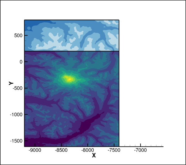
Source data.
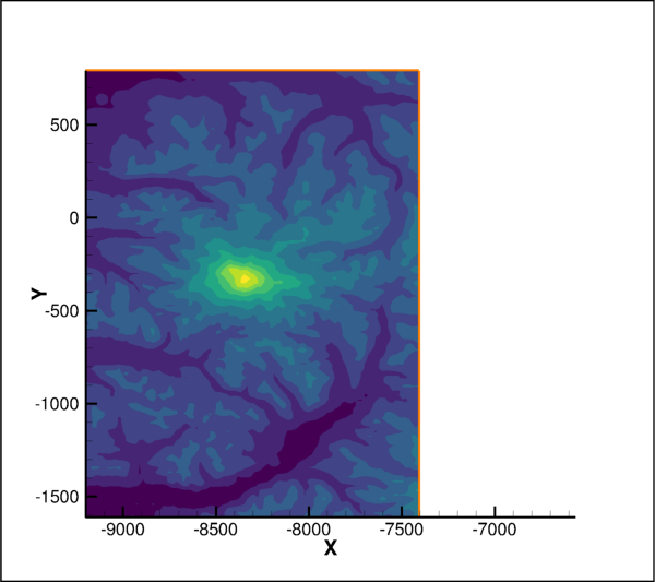
Interpolated data.
data.operate.interpolate_kriging()
- tecplot.data.operate.interpolate_kriging(destination_zone, source_zones=None, variables=None, krig_range=0.3, zero_value=0.0, drift=Drift.Linear, point_selection=PtSelection.OctantN, num_points=8, plot=None)[source]
Kriging interpolation onto a destination zone.
- Parameters:
destination_zone (zone or
int) – The destination zone (or zone index) for interpolation.source_zones (zones or
integers, optional) – Zones (or zone indices) used to obtain the field values for interpolation. By default, all zones except the destination_zone will be used. All source zones must be FE-Tetra, FE-Brick or IJK-ordered when doing kriging interpolation in 3D.variables (
variablesorintegers, optional) – Variables (or variable indices) to interpolate. By default, all variables except those assigned to the axes will be used and is in general dependent on the active plot type of the frame.krig_range (
float, optional) – Distance beyond which source points become insignificant. Must be between zero and one, inclusive. (default: 0.3)zero_value (
float, optional) – Semi-variance at each source data point on a normalized scale from zero to one. (default: 0.0)drift (
Drift, optional) – Overall trend for the data. Possible values:Drift.None_no trend,Drift.Linear(default) linear trend,Drift.Quadquadratic trend.point_selection (
PtSelection, optional) – Method for determining which source points to consider for each destination data point. Possible values:PtSelection.OctantN(default) closest num_points selected by coordinate-system octants,PtSelection.NearestNclosest num_points to the destination point,PtSelection.Allall points in the source zone.num_points (
int, optional) – Number of source points to consider for each destination data point if point_selection isPtSelection.OctantNorPtSelection.NearestN. (default: 8)plot (Plot, optional) – The plot to use when interpolating which determines the dimensionality and spatial variables. By default, the active plot on the active frame will be used.
Note
Cartesian 2D and 3D plots only.
This interpolation method relies on the coordinates, \((x, y)\) for 2D or \((x, y, z)\) for 3D, set for the active (or given) plot which must be either Cartesian2D or Cartesian3D.
The following example loads a 2D dataset and interpolates the first zone to a new one with a larger grid spacing:
import os
import numpy as np
import tecplot as tp
from tecplot.constant import *

# Use interpolation to merge information from two independent zones
examples_dir = tp.session.tecplot_examples_directory()
datafile = os.path.join(examples_dir, 'SimpleData',
                        'RainierElevation.plt')
dataset = tp.data.load_tecplot(datafile)
# Get list of source zones to use later
srczones = list(dataset.zones())

fr = tp.active_frame()
plot = fr.plot(PlotType.Cartesian2D)
plot.activate()
plot.show_contour = True
plot.show_edge = True

# Show two section of the plot independently
plot.contour(0).legend.show = False
plot.contour(1).legend.show = False
plot.contour(1).colormap_name = 'Diverging - Blue/Red'
for scrzone in srczones:
    plot.fieldmap(scrzone).edge.line_thickness = 0.4
plot.fieldmap(0).contour.flood_contour_group = plot.contour(1)

# export image of original data
tp.export.save_png('interpolate_2d_source.png', 600, supersample=3)

# use the first zone as the source, and get the range of (x, y)
xvar = plot.axes.x_axis.variable
yvar = plot.axes.y_axis.variable
ymin, xmin = 99999,99999
ymax, xmax = -99999,-99999
for scrzone in srczones:
    curxmin, curxmax = scrzone.values(xvar.index).minmax()
    curymin, curymax = scrzone.values(yvar.index).minmax()
    ymin = min(curymin,ymin)
    ymax = max(curymax,ymax)
    xmin = min(curxmin,xmin)
    xmax = max(curxmax,xmax)

# create new zone with a coarse grid
# onto which we will interpolate from the source zone
xpoints = 20
ypoints = 20
newzone = dataset.add_ordered_zone('Interpolated', (xpoints, ypoints))

# setup the (x, y) positions of the new grid
xx = np.linspace(xmin, xmax, xpoints)
yy = np.linspace(ymin, ymax, ypoints)
YY, XX = np.meshgrid(yy, xx, indexing='ij')
newzone.values(xvar.index)[:] = XX.ravel()
newzone.values(yvar.index)[:] = YY.ravel()

# perform linear interpolation from the source to the new zone
tp.data.operate.interpolate_kriging(newzone, source_zones=srczones,
                                    drift=Drift.None_, num_points=1)

# show the new zone's data, hide the source
plot.fieldmap(newzone).show = True
plot.fieldmap(newzone).contour.show = True
plot.fieldmap(newzone).contour.flood_contour_group = plot.contour(0)
plot.fieldmap(newzone).edge.show = True
plot.fieldmap(newzone).edge.line_thickness = .4
plot.fieldmap(newzone).edge.color = Color.Orange

for scrzone in srczones:
    plot.fieldmap(scrzone).show = False

# export image of interpolated data
tp.export.save_png('interpolate_krig_2d_dest.png', 600, supersample=3)
Source data.

Interpolated data.
data.operate.interpolate_linear()
- tecplot.data.operate.interpolate_linear(destination_zone, source_zones=None, variables=None, fill_value=None, plot=None)[source]
Linear interpolation onto a destination zone.
- Parameters:
destination_zone (zone or
int) – The destination zone (or zone index) for interpolation.source_zones (zones or
integers, optional) – Zones (or zone indices) used to obtain the field values for interpolation. By default, all zones except the destination_zone will be used. All source zones must be FE-Tetra, FE-Brick or be IJK-ordered when doing linear interpolation in 3D.variables (
variablesorintegers, optional) – Variables (or variable indices) to interpolate. By default, all variables except those assigned to the axes will be used and is in general dependent on the active plot type of the frame.fill_value (
float, optional) – Constant value to which all points outside the data field are set. By default, the values outside the field are preserved.plot (Plot, optional) – The plot to use when interpolating which determines the dimensionality and spatial variables. By default, the active plot on the active frame will be used.
Note
Cartesian 2D and 3D plots only.
This interpolation method relies on the coordinates, \((x, y)\) for 2D or \((x, y, z)\) for 3D, set for the active (or given) plot which must be either Cartesian2D or Cartesian3D.
The following example loads a 2D dataset and uses interpolation to merge information from two independent zones:
import os
import numpy as np
import tecplot as tp
from tecplot.constant import *

# Use interpolation to merge information from two independent zones
examples_dir = tp.session.tecplot_examples_directory()
datafile = os.path.join(examples_dir, 'SimpleData', 'RainierElevation.plt')
dataset = tp.data.load_tecplot(datafile)
# Get list of source zones to use later
srczones = list(dataset.zones())

fr = tp.active_frame()
plot = fr.plot(PlotType.Cartesian2D)
plot.activate()
plot.show_contour = True
plot.show_edge = True

# Show two section of the plot independently
plot.contour(0).legend.show = False
plot.contour(1).legend.show = False
plot.contour(1).colormap_name = 'Diverging - Blue/Red'
for scrzone in srczones:
    plot.fieldmap(scrzone).edge.line_thickness = 0.4
plot.fieldmap(0).contour.flood_contour_group = plot.contour(1)

# export image of original data
tp.export.save_png('interpolate_2d_source.png', 600, supersample=3)

# use the first zone as the source, and get the range of (x, y)
xvar = plot.axes.x_axis.variable
yvar = plot.axes.y_axis.variable
ymin, xmin = 99999,99999
ymax, xmax = -99999,-99999
for scrzone in srczones:
    curxmin, curxmax = scrzone.values(xvar.index).minmax()
    curymin, curymax = scrzone.values(yvar.index).minmax()
    ymin = min(curymin,ymin)
    ymax = max(curymax,ymax)
    xmin = min(curxmin,xmin)
    xmax = max(curxmax,xmax)

# create new zone with a coarse grid
# onto which we will interpolate from the source zone
xpoints = 40
ypoints = 40
newzone = dataset.add_ordered_zone('Interpolated', (xpoints, ypoints))

# setup the (x, y) positions of the new grid
xx = np.linspace(xmin, xmax, xpoints)
yy = np.linspace(ymin, ymax, ypoints)
YY, XX = np.meshgrid(yy, xx, indexing='ij')
newzone.values(xvar.index)[:] = XX.ravel()
newzone.values(yvar.index)[:] = YY.ravel()

# perform linear interpolation from the source to the new zone
tp.data.operate.interpolate_linear(newzone, source_zones=srczones)

# show the new zone's data, hide the source
plot.fieldmap(newzone).show = True
plot.fieldmap(newzone).contour.show = True
plot.fieldmap(newzone).contour.flood_contour_group = plot.contour(0)
plot.fieldmap(newzone).edge.show = True
plot.fieldmap(newzone).edge.line_thickness = .4
plot.fieldmap(newzone).edge.color = Color.Orange

for scrzone in srczones:
    plot.fieldmap(scrzone).show = False

# export image of interpolated data
tp.export.save_png('interpolate_linear_2d_dest.png', 600, supersample=3)
Source data.

Interpolated data.
data.operate.smooth()
- tecplot.data.operate.smooth(array, num_passes=1, weight=0.8, boundary_condition=BoundaryCondition.Fixed, frame=None)[source]
Smooth a field data
Arrayin the dataset.- Parameters:
array (
Array) – The field data to smooth.num_passes (
int, optional) – The number of smoothing passes to perform. (default: 1)weight (
float, optional) – The relaxation factor for each pass of smoothing. Must be a number between zero and one exclusively. Higher numbers indicate a greater smoothing effect. (default: 0.8)boundary_condition (
BoundaryCondition, optional) – The boundary condition by which to smooth. Possible values areBoundaryCondition.Fixed(default),BoundaryCondition.ZeroGradientandBoundaryCondition.Zero2nd.frame (
Frame, optional) – TheFramethat specifies the spatial variables to smooth over via the active plot. By default, the frame associated with the inputArrayobject will be used.
The data will be smoothed over the spatial variables set by the plot and is dependent on the active plot type of the associated
Frame(Cartesian2DorCartesian3D). Example usage:>>> tp.data.operate.smooth(dataset.zone('Zone').values('Pressure'))
data.operate.transform_polar_to_rectangular()
- tecplot.data.operate.transform_polar_to_rectangular(r, theta, x=None, y=None, angle_units=AngleUnits.Radians, zones=None)[source]
Transform all points from polar to rectangular coordinates.
- Parameters:
r (
Variable) – The radial input variable.theta (
Variable) – The angular input variable in angle_units from the \(x\)-axis.x (
Variable, optional) – The rectangular output \(x\) variable. By default, a new variable will be created. Both x and y must be specified together as either existing variables or asNone.y (
Variable, optional) – The rectangular output \(y\) variable. By default, a new variable will be created. Both x and y must be specified together as either existing variables or asNone.angle_units (
AngleUnits, optional) – The units of the angular variables. This may be eitherAngleUnits.Radians(default) orAngleUnits.Degrees.zones (
listof Zones, optional) – Specific zones to transform. By default, all zones are transformed.
This example will create two new variables in the dataset corresponding to the \(x\) and \(y\) equivalents of the \(r\) and \(theta\) variables:
>>> dataset = tp.active_frame().dataset
>>> r = dataset.variable('R (m)')
>>> theta = dataset.variable('Theta (rad)')
>>> tp.data.operate.transform_polar_to_rectangular(r, theta)
>>> x, y = dataset.variable(-2), dataset.variable(-1)
Warning
Source variables must have the same location as the destination variables.
The variables involved with this transformation must all be either nodal or cell-centered.
data.operate.transform_rectangular_to_polar()
- tecplot.data.operate.transform_rectangular_to_polar(x, y, r=None, theta=None, angle_units=AngleUnits.Radians, zones=None)[source]
Transform all points from rectangular to polar coordinates.
- Parameters:
x (
Variable) – The rectangular input \(x\) variable.y (
Variable) – The rectangular input \(y\) variable.r (
Variable, optional) – The radial output \(r\) variable. By default, a new variable will be created. Both r and theta must be specified together as either existing variables or asNone.theta (
Variable, optional) – The angular output \(theta\) variable. By default, a new variable will be created. Both r and theta must be specified together as either existing variables or asNone.angle_units (
AngleUnits, optional) – The units of the angular variables. This may be eitherAngleUnits.Radians(default) orAngleUnits.Degrees.zones (
listof Zones, optional) – Specific zones to transform. By default, all zones are transformed.
This example will create two new variables in the dataset corresponding to the \(r\) and \(theta\) equivalents of the \(x\) and \(y\) variables:
>>> dataset = tp.active_frame().dataset
>>> x = dataset.variable('X (m)')
>>> y = dataset.variable('Y (m)')
>>> tp.data.operate.transform_rectangular_to_polar(x, y)
>>> theta, r = dataset.variable(-2), dataset.variable(-1)
Warning
Source variables must have the same location as the destination variables.
The variables involved with this transformation must all be either nodal or cell-centered.
data.operate.transform_rectangular_to_spherical()
- tecplot.data.operate.transform_rectangular_to_spherical(x, y, z, r=None, theta=None, psi=None, angle_units=AngleUnits.Radians, zones=None)[source]
Transform all points from rectangular to spherical coordinates.
- Parameters:
x (
Variable) – The rectangular input \(x\) variable.y (
Variable) – The rectangular input \(y\) variable.z (
Variable) – The rectangular input \(z\) variable.r (
Variable, optional) – The radial output \(r\) variable. By default, a new variable will be created. All of r, theta and psi must be specified together as either existing variables or asNone.theta (
Variable, optional) – The angular output \(theta\) variable from the \(x\)-axis. By default, a new variable will be created. All of r, theta and psi must be specified together as either existing variables or asNone.psi (
Variable, optional) – The angular output \(psi\) variable from the \(z\)-axis. By default, a new variable will be created. All of r, theta and psi must be specified together as either existing variables or asNone.angle_units (
AngleUnits, optional) – The units of the angular variables. This may be eitherAngleUnits.Radians(default) orAngleUnits.Degrees.zones (
listof Zones, optional) – Specific zones to transform. By default, all zones are transformed.
This example will create three new variables in the dataset corresponding to the \((r, theta, psi)\) equivalents of the \((x, y, z)\) variables:
>>> dataset = tp.active_frame().dataset
>>> x = dataset.variable('X (m)')
>>> y = dataset.variable('Y (m)')
>>> z = dataset.variable('Z (m)')
>>> tp.data.operate.transform_rectangular_to_spherical(x, y, z)
>>> theta = dataset.variable(-3)
>>> r = dataset.variable(-2)
>>> psi = dataset.variable(-1)
Warning
Source variables must have the same location as the destination variables.
The variables involved with this transformation must all be either nodal or cell-centered.
data.operate.transform_spherical_to_rectangular()
- tecplot.data.operate.transform_spherical_to_rectangular(r, theta, psi, x=None, y=None, z=None, angle_units=AngleUnits.Radians, zones=None)[source]
Transform all points from spherical to rectangular coordinates.
- Parameters:
r (
Variable) – The radial input variable.theta (
Variable) – The angular input variable in angle_units from the \(x\)-axis.psi (
Variable) – The angular input variable in angle_units from the \(z\)-axis.x (
Variable, optional) – The rectangular output \(x\) variable. By default, a new variable will be created. All of x, y and z must be specified together as either existing variables or asNone.y (
Variable, optional) – The rectangular output \(y\) variable. By default, a new variable will be created. All of x, y and z must be specified together as either existing variables or asNone.z (
Variable, optional) – The rectangular output \(z\) variable. By default, a new variable will be created. All of x, y and z must be specified together as either existing variables or asNone.angle_units (
AngleUnits, optional) – The units of the angular variables. This may be eitherAngleUnits.Radians(default) orAngleUnits.Degrees.zones (
listof Zones, optional) – Specific zones to transform. By default, all zones are transformed.
This example will create three new variables in the dataset corresponding to the \((x, y, z)\) equivalents of the \((r, theta, psi)\) variables:
>>> dataset = tp.active_frame().dataset
>>> r = dataset.variable('R (m)')
>>> theta = dataset.variable('Theta (rad)')
>>> psi = dataset.variable('Psi (rad)')
>>> tp.data.operate.transform_spherical_to_rectangular(r, theta, psi)
>>> x = dataset.variable(-3)
>>> y = dataset.variable(-2)
>>> z = dataset.variable(-1)
Warning
Source variables must have the same location as the destination variables.
The variables involved with this transformation must all be either nodal or cell-centered.
Data Extractions
data.extract.extract_blanked_zones()
- tecplot.data.extract.extract_blanked_zones(*zones, **kwargs)[source]
Extract subsets of Zones based on blanking conditions of the plot.
- Parameters:
*zones (Zones, required) – Set of source zones to extract.
- Keyword Arguments:
plot (
Cartesian3DFieldPlotor other data-backed plot type, optional) – The plot that defines the blanking conditions. By default, the active plot will be used.- Returns:
A new zone will be created for each zone specified unless blanking dictates that all cells and points in the entire zone are blanked. The following example extracts all zones in the dataset:
import os

import tecplot as tp
from tecplot.constant import *

examples_dir = tp.session.tecplot_examples_directory()
datafile = os.path.join(examples_dir, 'SimpleData', 'VortexShedding.plt')

dataset = tp.data.load_tecplot(datafile)

plot = tp.active_frame().plot()
plot.show_contour = True

xax = plot.axes.x_axis
xax.min = -0.005
xax.max = 0.015
yax = plot.axes.y_axis
yax.min = -0.01
yax.max = 0.002

# Setup value blanking
vblank = plot.value_blanking
constraint = vblank.constraint(0)
constraint.variable_index = 1
constraint.comparison_operator = RelOp.GreaterThan
constraint.active = True
vblank.active = True

# Use list comprehension to get all zones assocaitated with
# a specific strand, in this case strand 1
in_zns = [zn for zn in dataset.zones() if zn.strand == 1]

# Extract all zones assocaitated with strand 1
ext_zns = tp.data.extract.extract_blanked_zones(in_zns)

# Place all extracted zones into the same strand
for zn in ext_zns:
    zn.strand = 2

# Turn off plotting for the original zone and turn on plotting
# of the extracted zones.
plot.fieldmap(0).show = False
plot.fieldmap(1).show = True

tp.export.save_time_animation_mpeg4('extract_blanked_zones.mp4',
                                    width=400, end_time=0.0004,
                                    supersample=3)
Added in version 2020.1: Extracting blanked zones requires Tecplot 360 2020 R1 or later.
data.extract.extract_line()
- tecplot.data.extract.extract_line(points, num_points=None, frame=None, dataset=None)[source]
Create new zone from a line in the dataset.
- Parameters:
points (
2D numeric array) – The points defining the line in two or three dimensions. This array must be of the shape (N, D) where N is the number points and D is the number of dimensions. That is, it must take the form[(x0, y0, z0), (x1, y1, z1) ...]. Points that do not lie within the dataset volume will be removed from the resulting zone.num_points (
int, optional) – The number of points to evenly distribute along the polyline. (default: length of points or N)frame (
Frame, optional) – AFramethat holds theDatasetto operate on which must match dataset if given. (default: currently activeFrame)dataset (
Dataset, optional) – TheDatasetto operate on which must be attached to frame if given. (default: currently activeDataset)
- Returns:
A 1D
OrderedZonerepresenting a line through the data. Points outside of the dataset will be removed from the extracted zone resulting in fewer points than input.
Warning
Line extraction is only available when the plot type is set to
Cartesian2DorCartesian3D:>>> from tecplot.constant import PlotType >>> frame.plot_type = PlotType.Cartesian3D
This example shows how to extract a zone along a line, overlaying the result in a new frame:
import numpy as np from os import path import tecplot as tp from tecplot.constant import * examples_dir = tp.session.tecplot_examples_directory() datafile = path.join(examples_dir, 'SimpleData', 'VortexShedding.plt') dataset = tp.data.load_tecplot(datafile) frame = tp.active_frame() frame.activate() plot = frame.plot() plot.contour(0).variable = dataset.variable("P(N/M2)") plot.show_contour = True plot.contour(0).levels.reset(num_levels=11) plot.contour(0).colormap_name = 'Sequential - Yellow/Green/Blue' plot.axes.y_axis.min = -0.01 plot.axes.y_axis.max = 0.01 plot.axes.x_axis.min = -0.005 plot.axes.x_axis.max = 0.015 xx = np.linspace(0, 0.01, 100) yy = np.zeros(100) line = tp.data.extract.extract_line(zip(xx, yy)) plot.show_mesh = True plot.fieldmap(0).mesh.show = False frame = tp.active_page().add_frame() frame.position = (3.0, 0.5) frame.height = 2 frame.width = 4 plot = tp.active_frame().plot(PlotType.XYLine) plot.activate() plot.delete_linemaps() lmap = plot.add_linemap('data', line, x=dataset.variable('P(N/M2)'), y=dataset.variable('T(K)')) lmap.line.line_thickness = 2.0 plot.axes.x_axis(0).title.font.size = 10 plot.axes.y_axis(0).title.font.size = 10 plot.axes.viewport.left = 20 plot.axes.viewport.bottom = 20 plot.view.fit() tp.export.save_png("extract_line.png", region=ExportRegion.AllFrames, width=600, supersample=3)
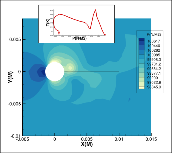
data.extract.extract_slice()
- tecplot.data.extract.extract_slice(origin=(0, 0, 0), normal=(0, 0, 1), source=None, mode=ExtractMode.SingleZone, copy_cell_centers=None, assign_strand_ids=None, transient_mode=TransientOperationMode.SingleSolutionTime, frame=None, dataset=None, resulting_1d_zone_type=Resulting1DZoneType.FELineSegment, **kw)[source]
Create new zone from a plane in the dataset.
- Parameters:
origin (array of three
floats) – Point in space, \((x, y, z)\), that lies on the slice plane.normal (array of three
floats) – Vector direction, \((x, y, z)\), indicating the normal of the slice plane.source (
SliceSource) – Source zone types to consider when extracting the slice. Possible values:SliceSource.LinearZones,SliceSource.SurfaceZones,SliceSource.SurfacesOfVolumeZones,SliceSource.VolumeZones(default).mode (
ExtractMode) – Controls how many zones are created. Possible values are:ExtractMode.SingleZone(default),ExtractMode.OneZonePerConnectedRegionandExtractMode.OneZonePerSourceZone.copy_cell_centers (
bool) – IfTrue, cell-center values will be copied when possible to the extracted slice plane. Cell-centers are copied when a variable is cell-centered for all the source zones through which the slice passes. Otherwise, extracted planes use node-centered data, which is calculated by interpolation. (default:False)assign_strand_ids (
bool) – Automatically assign strand IDs to the data extracted from transient sources. This is only available if multiple_zones isFalse. (default:True)transient_mode (
TransientOperationMode) – Determines which solution times are used to extract slices when transient data is available in the dataset. Possible values areTransientOperationMode.SingleSolutionTime(default) orTransientOperationMode.AllSolutionTimes.frame (
Frame, optional) – AFramethat holds theDatasetto operate on which must match dataset if given. (default: currently activeFrame)dataset (
Dataset, optional) – TheDatasetto operate on which must be attached to frame if given. (default: currently activeDataset)resulting_1d_zone_type (
Resulting1DZoneType, optional) – The type of zone to create when the result is one-dimensional. Possible values are:Resulting1DZoneType.FELineSegment(default) andResulting1DZoneType.IOrderedIfPossible.
- Returns:
Warning
Slicing is only available when the plot type is set to 3D:
>>> from tecplot.constant import PlotType
>>> frame.plot_type = PlotType.Cartesian3D
Note
The extracted zone is returned if mode is
ExtractMode.SingleZoneand transient_mode isTransientOperationMode.SingleSolutionTime, otherwise a generator of the extracted zones.See also
This example shows extracting a slice zone from the surface a wing:
import os
import tecplot as tp
from tecplot.constant import PlotType, SliceSource

examples_dir = tp.session.tecplot_examples_directory()
datafile = os.path.join(examples_dir, 'OneraM6wing',
                        'OneraM6_SU2_RANS.plt')
dataset = tp.data.load_tecplot(datafile)

frame = tp.active_frame()
frame.plot_type = PlotType.Cartesian3D

# set active plot to 3D and extract
# an arbitrary slice from the surface
# data on the wing
extracted_slice = tp.data.extract.extract_slice(
    origin=(0, 0.25, 0),
    normal=(0, 1, 0),
    source=SliceSource.SurfaceZones,
    dataset=dataset)

# switch plot type in current frame, clear plot
plot = frame.plot(PlotType.XYLine)
plot.activate()
plot.delete_linemaps()

# create line plot from extracted zone data
cp_linemap = plot.add_linemap(
    name='Quarter-chord C_p',
    zone=extracted_slice,
    x=dataset.variable('x'),
    y=dataset.variable('Pressure_Coefficient'))

# set style of linemap plot and
# update axes limits to show data
cp_linemap.line.color = tp.constant.Color.Blue
cp_linemap.line.line_thickness = 0.8
cp_linemap.y_axis.reverse = True
plot.view.fit()

# export image of pressure coefficient as a function of x
tp.export.save_png('wing_slice_pressure_coeff.png', 600, supersample=3)
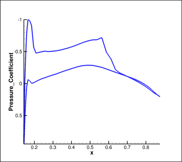
data.extract.extract_connected_regions()
- tecplot.data.extract.extract_connected_regions(*zones, **kwargs)[source]
Create new zones from regions of connected cells.
- Parameters:
*zones (Zones, required) – Source zones from which to extract connected regions. All source zones must be finite-element zones, either classic FE or polygonal/polyhedral.
- Keyword Arguments:
assign_strand_ids (
bool, optional) – Automatically assign strand IDs to the zones extracted from transient sources. If True the resulting zones will be all be assigned to the same newly created strand id. (default:True)frame (
Frame, optional) – AFramethat holds theDatasetto operate on which must match dataset if given. (default: currently activeFrame)dataset (
Dataset, optional) – TheDatasetto operate on which must be attached to frame if given. (default: currently activeDataset)
- Returns:
Added in version 2020.2: Extracting connected regions requires Tecplot 360 2020 R2 or later.
data.extract.triangulate()
- tecplot.data.extract.triangulate(*zones, **kwargs)[source]
Create a new zone by forming triangles from points in 2D zones.
- Parameters:
*zones (Zones) – Set of 2-dimensional source zones to triangulate.
- Keyword Arguments:
boundary_zones (
listof \(I\)-Ordered Zones, optional) – Set of \(I\)-ordered zones that define the boundaries across which no triangles can be created. (default:None)include_boundary_points (
bool, optional) – IfTrue, boundary points will be used to create triangles. (default:False)keep_factor (
floatin the range [0.0, 0.5], optional) – The smaller the number, the more likely it will be that highly obtuse triangles will be created opening toward the outside of the triangulated zone.plot (
Cartesian2DFieldPlot, optional) – The plot defining the \((x, y)\) variables in the dataset. If not set, the active plot will be used which must be of typeCartesian2DFieldPlot.
- Returns:
ClassicFEZone– The resulting triangulated zone.
The active plot or the plot specified must be of type
Cartesian2DFieldPlotand the boundary zones, if supplied, may only be \(I\)-ordered zones. This example creates a new zone by triangulating data points from two other Zones:>>> zone0 = dataset.zone('Zone 0') >>> zone1 = dataset.zone('Zone 1') >>> new_zone = tp.data.extract.triangulate(zone0, zone1)
Data Access
Dataset
- class tecplot.data.Dataset(uid, frame)[source]
Table of
Arraysidentified by Zone andVariable.This is the primary data container within the Tecplot Engine. A
Datasetcan be shared among severalFrames, though any particularDatasetobject will have a handle to at least one of them. Any modification of a sharedDatasetwill be reflected in allFramesthat use it.Though a
Datasetis usually attached to aFrameand the plot style associated with that, it can be thought of as independent from any style or plotting representation. EachDatasetconsists of a list ofVariableswhich are used by one or more of a list of Zones. TheVariabledetermines the data type, while the Zone determines the layout such as shape and ordered vs unordered.The actual data are found at the intersection of a Zone and
Variableand the resulting object is anArray. The data array can be obtained using either path:>>> # These two lines obtain the same object "x" >>> x = dataset.zone('My Zone').values('X') >>> x = dataset.variable('X').values('My Zone')
A
Datasetis the object returned by most data-loading operations in PyTecplot:>>> dataset = tecplot.data.load_tecplot('my_data.plt')
Under
Dataset, there are a number methods to create and delete Zones andvariables.Attributes
A
collections.namedtupleobject using variable names.Auxiliary data for this dataset.
Number of solution times in the dataset.
Solution time clustering options.
Solution times in the dataset.
A
listof names for all variables in the dataset.A
listof names for all zones in the dataset.Methods
add_fe_mixed_zone(name, num_points, ...)Add a finite-element Zone consisting of one or more blocks of uniform cell-type (sections).
add_fe_zone(zone_type, name, num_points, ...)add_ordered_zone(name, shape, **kwargs)add_poly_zone(zone_type, name, num_points, ...)add_variable(name[, dtypes, locations])add_zone(zone_type, name, shape[, dtypes, ...])branch_connectivity(zones)Breaks connectivity sharing between zones.
branch_variables(zones, variables[, copy_data])Breaks data sharing between zones.
copy_zones(*zones, **kwargs)delete_variables(*variables)delete_zones(*zones)mirror_zones(mirror_variables, *zones)share_connectivity(source_zone, ...)Share connectivity between zones.
share_variables(source_zone, ...)Share field data between zones.
variable(pattern)Returns the
Variableby index or string pattern.variables([pattern])Yields all
Variablesmatching a pattern.zone(pattern)Returns Zone by index or string pattern.
zones([pattern])Yields all Zones matching a pattern.
- Dataset.VariablesNamedTuple
A
collections.namedtupleobject using variable names.The variable names are transformed to be unique, valid identifiers suitable for use as the key-list for a
collections.namedtuple. This means that all invalid characters such as spaces and dashes are converted to underscores, Python keywords are appended by an underscore, leading numbers or empty names are prepended with a “v” and duplicate variable names are indexed starting with zero, padded left with zeros variable names duplicated more than nine times. The following table gives some specific examples:Variable names
Resulting namedtuple fields
'x', 'y''x', 'y''x', 'x''x0', 'x1''X', 'Y=f(X)''X', 'Y_f_X_''x 2', '_', '_''x_2', 'v0', 'v1''def', 'if''def_', 'if_''1', '2', '3''v1', 'v2', 'v3'This example shows how one can use this n-tuple type with the result from a call to
tecplot.data.query.probe_at_position:from os import path import tecplot as tp examples_dir = tp.session.tecplot_examples_directory() datafile = path.join(examples_dir,'SimpleData','DownDraft.plt') dataset = tp.data.load_tecplot(datafile) result = tp.data.query.probe_at_position(0,0.1,0.3) data = dataset.VariablesNamedTuple(*result.data) # prints: (RHO, E) = (1.17, 252930.37) msg = '(RHO, E) = ({:.2f}, {:.2f})' print(msg.format(data.RHO, data.E))
- Dataset.add_fe_mixed_zone(name, num_points, sections, **kwargs)[source]
Add a finite-element Zone consisting of one or more blocks of uniform cell-type (sections).
- Parameters:
name (
str) – have to be unique.num_points (
int) – Number of points (nodes) in this zone.sections (
listortuples) – A list of the properties of the sections in the form:(num_elements, cell_shape, grid_order, basis_function). The grid_order and basis_func items may be omitted and will default to 1 (linear) andFECellBasisFunction.Lagrangianrespectively.**kwargs – These arguments are passed to
Dataset.add_zone.
See also
Keyword arguments are passed to the parent zone creation method
Dataset.add_zone.Warning
Setting connectivity in connected mode.
When connected to a running instance of Tecplot 360 using the TecUtil Server, care must be taken to ensure that the GUI does not try to render the data between the creation of the zone and the setting of the connectivity, through the
FacemaporNodemapobjects. This can be achieved by setting the plot type of the frame(s) holding on to the dataset toPlotType.Sketchbefore creating the zone and only going toPlotType.Cartesian3Dafter the connectivity is set. Tecplot 360 may get into a bad state, corrupting loaded data, if it attempts to render (especially polytope) data without connectivity.Warning
Variable Sharing.
If a new zone has the same type and shape as an existing zone, variables may be shared by Tecplot to conserve memory. This variable sharing can be broken with the
branch_variables()method. More information on when variable sharing occurs can be found in the Tecplot User’s Manual.Note
Performance considerations for data manipulations.
When performing many data-manipulation operations including adding zones, adding variables, modifying field data or connectivity, and especially in connected mode, it is recommended to do this all with the
tecplot.session.suspend(). This will prevent the Tecplot engine from trying to “keep up” with the changes. Tecplot will be notified of all changes made upon exit of this context. This may result in significant performance gains for long operations.For more details, see the “working with datasets” examples shipped with PyTecplot in the Tecplot 360 distribution.
- Dataset.add_fe_zone(zone_type, name, num_points, num_elements, **kwargs)[source]
Add a single finite-element Zone to this
Dataset.- Parameters:
zone_type (
ZoneType) – created. Possible values are:FETriangle,FEQuad,FETetra,FEBrickandFELineSeg.name (
str) – does not have to be unique.num_points (
int) – Number of points (nodes) in this zone.num_elements (
int) – Number of elements in this zone. The nodemap will have the shape (num_points, num_elements).**kwargs – These arguments are passed to
Dataset.add_zone.
See also
Keyword arguments are passed to the parent zone creation method
Dataset.add_zone.Warning
Setting connectivity in connected mode.
When connected to a running instance of Tecplot 360 using the TecUtil Server, care must be taken to ensure that the GUI does not try to render the data between the creation of the zone and the setting of the connectivity, through the
FacemaporNodemapobjects. This can be achieved by setting the plot type of the frame(s) holding on to the dataset toPlotType.Sketchbefore creating the zone and only going toPlotType.Cartesian3Dafter the connectivity is set. Tecplot 360 may get into a bad state, corrupting loaded data, if it attempts to render (especially polytope) data without connectivity.Warning
Variable Sharing.
If a new zone has the same type and shape as an existing zone, variables may be shared by Tecplot to conserve memory. This variable sharing can be broken with the
branch_variables()method. More information on when variable sharing occurs can be found in the Tecplot User’s Manual.Note
Performance considerations for data manipulations.
When performing many data-manipulation operations including adding zones, adding variables, modifying field data or connectivity, and especially in connected mode, it is recommended to do this all with the
tecplot.session.suspend(). This will prevent the Tecplot engine from trying to “keep up” with the changes. Tecplot will be notified of all changes made upon exit of this context. This may result in significant performance gains for long operations.The number of points (also known as nodes) per finite-element is determined from the
zone_typeparameter. The follow table shows the number of points per element for the available zone types along with the resulting shape of the nodemap based on the number of points specified (\(N\)):Zone Type
Points/Element
Nodemap Shape
FELineSeg2
(\(N\), \(2 N\))
FETriangle3
(\(N\), \(3 N\))
FEQuad4
(\(N\), \(4 N\))
FETetra4
(\(N\), \(4 N\))
FEBrick8
(\(N\), \(8 N\))
For more details, see the “working with datasets” examples shipped with PyTecplot in the Tecplot 360 distribution.
- Dataset.add_ordered_zone(name, shape, **kwargs)[source]
Add a single ordered Zone to this
Dataset.- Parameters:
See also
Keyword arguments are passed to the parent zone creation method
Dataset.add_zone.Note
Performance considerations for data manipulations.
When performing many data-manipulation operations including adding zones, adding variables, modifying field data or connectivity, and especially in connected mode, it is recommended to do this all with the
tecplot.session.suspend(). This will prevent the Tecplot engine from trying to “keep up” with the changes. Tecplot will be notified of all changes made upon exit of this context. This may result in significant performance gains for long operations.This example creates a 10x10x10 ordered zone of double-precision floating-point numbers:
>>> from tecplot.constant import FieldDataType
>>> my_zone = dataset.add_zone('My Zone', (10, 10, 10),
...                            dtypes=FieldDataType.Double)
Here is a full example:
import numpy as np
import tecplot as tp
from tecplot.constant import PlotType, Color

# Generate data
x = np.linspace(-4, 4, 100)

# Setup Tecplot dataset
dataset = tp.active_frame().create_dataset('Data', ['x', 'y'])

# Create a zone
zone = dataset.add_ordered_zone('sin(x)', len(x))
zone.values('x')[:] = x
zone.values('y')[:] = np.sin(x)

# Create another zone
zone = dataset.add_ordered_zone('cos(x)', len(x))
zone.values('x')[:] = x
zone.values('y')[:] = np.cos(x)

# And one more zone
zone = dataset.add_ordered_zone('tan(x)', len(x))
zone.values('x')[:] = x
zone.values('y')[:] = np.tan(x)

# Set plot type to XYLine
plot = tp.active_frame().plot(PlotType.XYLine)
plot.activate()

# Show all linemaps and make the lines a bit thicker
for lmap in plot.linemaps():
    lmap.show = True
    lmap.line.line_thickness = 0.6

plot.legend.show = True

tp.export.save_png('add_ordered_zones.png', 600, supersample=3)
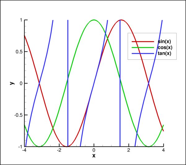
- Dataset.add_poly_zone(zone_type, name, num_points, num_elements, num_faces, **kwargs)[source]
Add a single polygonal Zone to this
Dataset.- Parameters:
zone_type (
ZoneType) – created. Possible values are:FEPolyhedronandFEPolygon.name (
str) – does not have to be unique.num_points (
int) – Number of points in this zone.num_elements (
int) – Number of elements in this zone.num_faces (
int) – Number of faces in this zone.**kwargs – These arguments are passed to
Dataset.add_zone.
See also
Keyword arguments are passed to the parent zone creation method
Dataset.add_zone.Warning
Setting connectivity in connected mode.
When connected to a running instance of Tecplot 360 using the TecUtil Server, care must be taken to ensure that the GUI does not try to render the data between the creation of the zone and the setting of the connectivity, through the
FacemaporNodemapobjects. This can be achieved by setting the plot type of the frame(s) holding on to the dataset toPlotType.Sketchbefore creating the zone and only going toPlotType.Cartesian3Dafter the connectivity is set. Tecplot 360 may get into a bad state, corrupting loaded data, if it attempts to render (especially polytope) data without connectivity.Warning
Variable Sharing.
If a new zone has the same type and shape as an existing zone, variables may be shared by Tecplot to conserve memory. This variable sharing can be broken with the
branch_variables()method. More information on when variable sharing occurs can be found in the Tecplot User’s Manual.Note
Performance considerations for data manipulations.
When performing many data-manipulation operations including adding zones, adding variables, modifying field data or connectivity, and especially in connected mode, it is recommended to do this all with the
tecplot.session.suspend(). This will prevent the Tecplot engine from trying to “keep up” with the changes. Tecplot will be notified of all changes made upon exit of this context. This may result in significant performance gains for long operations.Note
The num_faces is the number of unique faces.
The number of unique faces, given an element map can be obtained using the following function for polygon data:
def num_unique_faces(elementmap):
    return len(set( tuple(sorted([e[i], e[(i+1)%len(e)]]))
                for e in elementmap for i in range(len(e)) ))
This function creates a unique set of node pairs (edges around the polygons) and counts them. For polyhedron data, the following can be used:
def num_unique_faces(elementmap):
    return len(set( tuple(sorted(f)) for e in elementmap
                                     for f in e ))
which merely counts the number of unique faces defined in the element map.
For more details, see the “working with datasets” examples shipped with PyTecplot in the Tecplot 360 distribution.
- Dataset.add_variable(name, dtypes=None, locations=None)[source]
Add a single
Variableto the activeDataset.- Parameters:
name (
str) – The name of the newVariable. This does not have to be unique.dtypes (
FieldDataTypeorlistofFieldDataType, optional) – Data types of thisVariablefor each Zone in the currently activeDataset. Options are:FieldDataType.Float,Double,Int32,Int16,ByteandBit. If a single value, this will be duplicated for all Zones. (default:None)locations (
ValueLocationorlistofValueLocation, optional) – Point locations of thisVariablefor each Zone in the currently activeDataset. Options are:NodalandCellCentered. If a single value, this will be duplicated for all Zones. (default:None)
- Returns:
Note
Performance considerations for data manipulations.
When performing many data-manipulation operations including adding zones, adding variables, modifying field data or connectivity, and especially in connected mode, it is recommended to do this all with the
tecplot.session.suspend(). This will prevent the Tecplot engine from trying to “keep up” with the changes. Tecplot will be notified of all changes made upon exit of this context. This may result in significant performance gains for long operations.The added
Variablewill be available for use in each Zone of the dataset. This method should be used in conjunction with other data creation methods such asDataset.add_zone:import math import tecplot as tp from tecplot.constant import PlotType # Setup Tecplot dataset dataset = tp.active_frame().create_dataset('Data') dataset.add_variable('x') dataset.add_variable('s') zone = dataset.add_ordered_zone('Zone', 100) # Fill the dataset x = [0.1 * i for i in range(100)] zone.values('x')[:] = x zone.values('s')[:] = [math.sin(i) for i in x] # Set plot type to XYLine tp.active_frame().plot(PlotType.XYLine).activate() tp.export.save_png('add_variables.png', 600, supersample=3)
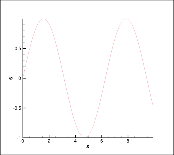
- Dataset.add_zone(zone_type, name, shape, dtypes=None, locations=None, face_neighbor_mode=None, parent_zone=None, solution_time=None, strand_id=None, index=None, sections=None)[source]
Add a single Zone to this
Dataset.- Parameters:
zone_type (
ZoneType) – created. Possible values are:Ordered,FETriangle,FEQuad,FETetra,FEBrick,FELineSeg,FEPolyhedron,FEPolygonandFEMixed.name (
str) – does not have to be unique.shape (
intorlistofintegers) – Specifies the length and dimension (up to three) of the new Zone. A 1D Zone is assumed if a singleintis given. This is (i, j, k) for ordered Zones, (num_points, num_elements) for finite-element Zones and (num_points, num_elements, num_faces) for polytope Zones where the number of faces is known.dtypes (
FieldDataType,listofFieldDataType, optional) – Data types of this Zone for eachVariablein the currently activeDataset. Options are:Float,Double,Int32,Int16,ByteandBit. If a single value, this will be duplicated for allVariables. IfNonethen the type of the firstVariable, defaulting toFieldDataType.Float, is used for all. (default:None)locations (
ValueLocation,listofValueLocation, optional) – Point locations of this Zone for eachVariablein the currently activeDataset. Options are:NodalandCellCentered. If a single value, this will be duplicated for allVariables. IfNonethen the type of the firstVariable, defaulting toNodal, is used for all. (default:None)face_neighbor_mode (
FaceNeighborMode, optional) – Specifies the face-neighbor mode for this zone. Options are:FaceNeighborMode.LocalOneToOne(default),FaceNeighborMode.LocalOneToMany,FaceNeighborMode.GlobalOneToOneorFaceNeighborMode.GlobalOneToMany.parent_zone (Zone, optional) – A parent Zone to be used when generating surface-restricted streamtraces.
solution_time (
float, optional) – Solution time for this zone. (default: 0)strand_id (
int, optional) – Associate this new Zone with a particular strand.index (
int, optional) – Number of the zone to add or replace. If omitted or set toNone, the new zone will be appended to the dataset. This value can be set to the number of a zone that already exists thereby replacing the existing zone. (default:None)sections (
listortuples) – A list of the properties of the sections in the form:(num_element, cell_shape, grid_order, basis_function). The grid_order and basis_func items may be omitted and will default to 1 (linear) andFECellBasisFunction.Lagrangianrespectively. This parameter is only used when zone_type is set toFEMixed.
- Returns:
Warning
Setting connectivity in connected mode.
When connected to a running instance of Tecplot 360 using the TecUtil Server, care must be taken to ensure that the GUI does not try to render the data between the creation of the zone and the setting of the connectivity, through the
FacemaporNodemapobjects. This can be achieved by setting the plot type of the frame(s) holding on to the dataset toPlotType.Sketchbefore creating the zone and only going toPlotType.Cartesian3Dafter the connectivity is set. Tecplot 360 may get into a bad state, corrupting loaded data, if it attempts to render (especially polytope) data without connectivity.Warning
Variable Sharing.
If a new zone has the same type and shape as an existing zone, variables may be shared by Tecplot to conserve memory. This variable sharing can be broken with the
branch_variables()method. More information on when variable sharing occurs can be found in the Tecplot User’s Manual.Note
Performance considerations for data manipulations.
When performing many data-manipulation operations including adding zones, adding variables, modifying field data or connectivity, and especially in connected mode, it is recommended to do this all with the
tecplot.session.suspend(). This will prevent the Tecplot engine from trying to “keep up” with the changes. Tecplot will be notified of all changes made upon exit of this context. This may result in significant performance gains for long operations.The added Zone will be able to use all
Variablesdefined in the dataset. This method should be used in conjunction with other data creation methods such asFrame.create_dataset. Example usage:>>> from tecplot.constant import ZoneType >>> zone = dataset.add_zone(ZoneType.Ordered, 'Zone', (10, 10, 10))
Note
The relationship and meaning of this method’s parameters change depending on the type of zone being created. Therefore, it is recommended to use the more specific zone creation methods:
- Dataset.aux_data
Auxiliary data for this dataset.
- Returns:
This is the auxiliary data attached to the dataset. Such data is written to the layout file by default and can be retrieved later. Example usage:
>>> frame = tp.active_frame()
>>> aux = frame.dataset.aux_data
>>> aux['Result'] = '3.14159'
>>> print(aux['Result'])
3.14159
- Dataset.branch_connectivity(zones)[source]
Breaks connectivity sharing between zones.
See also
Example usage:
>>> z = dataset.zone('My Zone')
>>> zcopy = z.copy()
>>> print([zn.index for zn in z.shared_connectivity])
[0,1]
>>> dataset.branch_connectivity(zcopy)
>>> print([zn.index for zn in z.shared_connectivity])
[]
- Dataset.branch_variables(zones, variables, copy_data=True)[source]
Breaks data sharing between zones.
- Parameters:
See also
Variable sharing allows you to lower the use of physical memory (RAM). When sharing a variable the memory used by the source zone is shared with the copied zone. Alterations to the variable in one zone will affect the other. Example usage:
>>> z = dataset.zone('My Zone')
>>> zcopy = z.copy(share_variables=True)
>>> print([zn.index for zn in z.values(0).shared_zones])
[0,1]
>>> dataset.branch_variables(zcopy,dataset.variable(0))
>>> print([zn.index for zn in z.values(0).shared_zones])
[]
>>> print([zn.index for zn in z.values(1).shared_zones])
[0,1]
- Dataset.copy_zones(*zones, **kwargs)[source]
Copies Zones within this
Dataset.- Parameters:
*zones (Zone, optional) – Specific Zones to copy. All zones will be copied if none are supplied.
share_variables (
boolorlistofVariables) – Share all variables between the original and generated zones ifTrueor the list of Variables to be shared. Variable sharing allows you to lower the use of physical memory (RAM). When sharing a variable the memory used by the source zone is shared with the copied zone. Alterations to the variable in one zone will affect the other. See alsoDataset.branch_variables(). Default:False.i_range (
tupleofintegers, optional) – Range (min, max, step) along theidimension for ordered data. Min and max are zero-based indicies where max is inclusive. If step causes max to be skipped, max will be included. IfNone(default), the entire range will be copied.j_range (
tupleofintegers, optional) – Range (min, max, step) along thejdimension for ordered data. Min and max are zero-based indicies where max is inclusive. If step causes max to be skipped, max will be included. IfNone(default), the entire range will be copied.k_range (
tupleofintegers, optional) – Range (min, max, step) along thekdimension for ordered data. Min and max are zero-based indicies where max is inclusive. If step causes max to be skipped, max will be included. IfNone(default), the entire range will be copied.
- Returns:
Note
Performance considerations for data manipulations.
When performing many data-manipulation operations including adding zones, adding variables, modifying field data or connectivity, and especially in connected mode, it is recommended to do this all with the
tecplot.session.suspend(). This will prevent the Tecplot engine from trying to “keep up” with the changes. Tecplot will be notified of all changes made upon exit of this context. This may result in significant performance gains for long operations.import tecplot as tp ds = tp.active_page().add_frame().create_dataset('D', ['x','y','z']) z = ds.add_ordered_zone('Z1', (3,3,3)) ds.copy_zones(z, i_range=(1, -1, 2), share_variables=True)
- Dataset.delete_variables(*variables)[source]
Remove
Variablesfrom thisDataset.>>> print(dataset.variable_names) ['X','Y','Z'] >>> dataset.delete_variables(dataset.variable('Z')) >>> print(dataset.variable_names) ['X','Y']
Warning
Deleting
Variablesinvalidates iterators referencing them in the containingDatasetsuch as those obtained fromDataset.variables(). It is recommended to create a list of theVariablesyou want to delete and to pass that into a single call toDataset.delete_variables()Notes
Multiple
Variablescan be deleted at once, though the lastVariablecan not be deleted. The following example deletes all but the firstVariablein theDataset(usuallyX):>>> # Try to delete all variables: >>> dataset.delete_variables(dataset.variables()) >>> # Dataset requires at least one variable to >>> # exist, so it leaves the first one: >>> print(dataset.variable_names) ['X']
- Dataset.delete_zones(*zones)[source]
Remove Zones from this
Dataset.>>> print(dataset.zone_names) ['Zone 1', 'Zone 2'] >>> dataset.delete_zones(dataset.zone('Zone 2')) >>> print(dataset.zone_names) ['Zone 1']
Warning
Deleting Zones invalidates iterators referencing them in the containing
Datasetsuch as those obtained fromDataset.zones(). It is recommended to create a list of the Zones you want to delete and to pass that into a single call toDataset.delete_zones()Notes
Multiple Zones can be deleted at once, though the last Zone can not be deleted. The following example deletes all but the first Zone in the
Dataset:>>> dataset.delete_zones(dataset.zones())
- Dataset.mirror_zones(mirror_variables, *zones)[source]
Mirrors Zones within this
Dataset.Each mirror zone has a name of the form “Mirror of zone sourcezone”, where sourcezone is the number of the zone from which the mirrored zone was created. The variables in the newly created zones are shared with their corresponding source zones, except for variables to be mirrored as specified.
- Parameters:
mirror_variables (
VariableorlistofVariables) – Variables in the new zone to be multiplied by \(-1\) after the zone is copied. the variables may beVariableobjects,strnames orintindices.*zones (Zones, optional) – Specific Zones to mirror. All zones will be mirrored if none are supplied. The values may also be
strnames orintindices.
- Returns:
Generator of mirrored zones.
This example show how to mirror all zones across the xy-plane in 3D:
>>> mirrored_zones = dataset.mirror_zones('Z')
- Dataset.num_solution_times
Number of solution times in the dataset.
This property is read-only. Solution times are grouped according to the current solution time clustering settings (see
Dataset.solution_time_clustering). Example usage:>>> print(dataset.num_solution_times) 10
Added in version 2017.3: Solution time manipulation requires Tecplot 360 2017 R3 or later.
- Type:
int(read-only)
- Dataset.num_variables
int: Number ofVariablesin thisDataset.This count includes disabled variables which were skipped when the data was loaded. Example usage:
>>> for i in range(dataset.num_variables):
...     variable = dataset.variable(i)
- Dataset.num_zones
int: Number of Zones in thisDataset.This count includes disabled zones which were skipped when loading the data. Example usage:
>>> for i in range(dataset.num_zones):
...     zone = dataset.zone(i)
Share connectivity between zones.
This method links the connectivity (
nodemaporfacemap) of the destination zones to the connectivity of the source zone. Modifying the connectivity of one zone will affect all others in this group.- Parameters:
See also
Example usage:
>>> z = dataset.zone('My Zone')
>>> zcopy = z.copy()
>>> print([zn.index for zn in z.shared_connectivity])
[0,1]
>>> dataset.branch_connectivity(zcopy)
>>> print([zn.index for zn in z.shared_connectivity])
[]
>>> dataset.share_connectivity(z,zcopy)
>>> print([zn.index for zn in z.shared_connectivity])
[0,1]
Share field data between zones.
This method links the underlying data
arraysof the destination zones to the data of the source zone. Modifying the array data of one zone will affect all others in this group.- Parameters:
See also
Example usage:
>>> z = dataset.zone('My Zone')
>>> zcopy = z.copy(share_variables=False)
>>> print([zn.index for zn in z.values(0).shared_zones])
[]
>>> dataset.share_variables(zcopy,[z],[dataset.variable(0)])
>>> print([zn.index for zn in z.values(0).shared_zones])
[0,1]
>>> print([zn.index for zn in z.values(1).shared_zones])
[]
- Dataset.solution_time_clustering
Solution time clustering options.
Example usage:
>>> from tecplot.constant import TimeScaling
>>> dataset.solution_time_clustering.time_scaling = \
...     TimeScaling.Logarithmic
Added in version 2021.2: Solution time clustering requires Tecplot 360 2021 R2 or later.
- Type:
- Dataset.solution_times
Solution times in the dataset.
This property is read-only. Solution times are grouped according to the current solution time clustering settings (see
Dataset.solution_time_clustering). Example usage:>>> print(dataset.solution_times) [0.0, 1.0, 2.0, 3.0, 4.0, 5.0, 6.0, 7.0, 8.0, 9.0]
Added in version 2017.3: Solution time manipulation requires Tecplot 360 2017 R3 or later.
- Dataset.title
-
Example usage:
>>> dataset.title = 'My Data'
Changed in version 2017.3: of Tecplot 360 The dataset title property requires Tecplot 360 2017 R3 or later.
- Dataset.variable(pattern)[source]
Returns the
Variableby index or string pattern.- Parameters:
pattern (
int,strorre.Pattern) – Zero-based index, case-insensitiveglob-style pattern stringor a compiledregex pattern instanceused to match the variable by name. A negative index is interpreted as counting from the end of the available variable.- Returns:
- Raises:
Note
A
Datasetcan containvariableswith identical names and only the first match found is returned. This is not guaranteed to be deterministic and care should be taken to have onlyvariableswith unique names when this feature is used.The
Variable.nameattribute is used to match the pattern to the desiredVariablethough this is not necessarily unique:>>> ds = frame.dataset >>> print(ds) Dataset: Zones: ['Rectangular zone'] Variables: ['x', 'y', 'z'] >>> x = ds.variable('x') >>> x == ds.variable(0) True
Warning
Zone and variable ordering may change between releases
Due to possible changes in data loaders or data formats over time, the ordering of zones and variables may be different between versions of Tecplot 360. Therefore it is recommended to always reference zones and variables by name instead of by index.
- Dataset.variable_names
A
listof names for all variables in the dataset.Warning
Newlines in string identifiers may affect performance.
When iterating over many items by name, such as must be done when fetching an item via pattern matching, PyTecplot will optimize the search only if there are no newline characters in the searched items. Iterating over strings that contain newlines will be slower and therefore, it is best to avoid using newlines in string identifiers or names of objects such as Zones or
Variables.Example usage:
>>> print(dataset.variable_names)
['x', 'y', 'z', 's']
- Dataset.variables(pattern=None)[source]
Yields all
Variablesmatching a pattern.- Parameters:
pattern (
strorre.Pattern, optional) – Case-insensitiveglob-style pattern stringor a compiledregex pattern instanceused to match variable names.- Returns:
Generator of
Variables. AllVariablesif pattern is not specified.
Example using case-insensitive glob-style matching:
>>> for variable in dataset.variables('A*'):
...     array = variable.values('My Zone')
Example using (case-sensitive) regex:
>>> import re
>>> for variable in dataset.variables(re.compile(r'A.*')):
...     array = variable.values('My Zone')
Warning
Zone and variable ordering may change between releases
Due to possible changes in data loaders or data formats over time, the ordering of zones and variables may be different between versions of Tecplot 360. Therefore it is recommended to always reference zones and variables by name instead of by index.
- Dataset.zone(pattern)[source]
Returns Zone by index or string pattern.
- Parameters:
pattern (
int,strorre.Pattern) – Zero-based index, case-insensitiveglob-style pattern stringor a compiledregex pattern instanceused to match the zones by name. A negative index is interpreted as counting from the end of the available zones.- Returns:
OrderedZone,ClassicFEZoneorPolyFEZonedepending on the zone type,Noneno matching zone name was found.- Raises:
Note
A
Datasetcan contain zones with identical names and only the first match found is returned. This is not guaranteed to be deterministic and care should be taken to have only zones with unique names when this feature is used.The
Zone.nameattribute is used to match the pattern to the desired Zone though this is not necessarily unique:>>> ds = frame.dataset >>> print(ds) Dataset: Zones: ['Rectangular zone'] Variables: ['x', 'y', 'z'] >>> rectzone = ds.zone('Rectangular zone') >>> rectzone == ds.zone(0) True
Warning
Zone and variable ordering may change between releases
Due to possible changes in data loaders or data formats over time, the ordering of zones and variables may be different between versions of Tecplot 360. Therefore it is recommended to always reference zones and variables by name instead of by index.
- Dataset.zone_names
A
listof names for all zones in the dataset.Warning
Newlines in string identifiers may affect performance.
When iterating over many items by name, such as must be done when fetching an item via pattern matching, PyTecplot will optimize the search only if there are no newline characters in the searched items. Iterating over strings that contain newlines will be slower and therefore, it is best to avoid using newlines in string identifiers or names of objects such as Zones or
Variables.Example usage:
>>> print(dataset.zone_names)
['Zone A', 'Zone B', 'Zone C']
- Dataset.zones(pattern=None)[source]
Yields all Zones matching a pattern.
- Parameters:
pattern (
strorre.Pattern, optional) – Case-insensitiveglob-style pattern stringor a compiledregex pattern instanceused to match zone names.- Returns:
Generator of
OrderedZones,ClassicFEZonesorPolyFEZonesdepending on the zone types. All zones if pattern is not specified.
If pattern is a string, this will be interpreted as a case-insensitive
glob-style pattern. Example using glob which will match all zones starting with “A” or “a”:>>> for zone in dataset.zones('A*'): ... x_array = zone.variable('X')
Alternatively, a regular-expression may be compiled using
re.compilewhich will be used directly. This example shows a case-sensitive regex search:>>> import re >>> pattern = re.compile('[A-Z]*') >>> for zone in dataset.zones(pattern): ... x_array = zone.variable('X')
Use list comprehension to construct a list of all zones with ‘Wing’ in the zone name. In contrast to the
Dataset.zones()method, this is case-sensitive:>>> wing_zones = [Z for Z in dataset.zones() if 'Wing' in Z.name]
Warning
Zone and variable ordering may change between releases
Due to possible changes in data loaders or data formats over time, the ordering of zones and variables may be different between versions of Tecplot 360. Therefore it is recommended to always reference zones and variables by name instead of by index.
SolutionTimeClustering
- class tecplot.data.SolutionTimeClustering(dataset)[source]
Settings for controlling solution time clustering of solution times.
By default, a dataset’s zones solution times are organized into time steps with the assumption that they are distributed linearly, and are grouped together if they are within the following solution time tolerance:
(tolerance_factor)*(max_time - min_time) + absolute_tolerance
Where by default the tolerance_factor is 1.0e-6 and the absolute_tolerance is 0.0.
Attributes
Absolute tolerance used to cluster zones by their solution times.
Scaling used to cluster zones by their solution times.
Tolerance factor used to cluster zones by solution times.
- SolutionTimeClustering.absolute_tolerance
Absolute tolerance used to cluster zones by their solution times.
Absolute tolerance applied to each solution time when clustering with nearby times. (Default: 0.0)
Example usage:
>>> dataset.solution_time_clustering.absolute_tolerance = 0.0025
Added in version 2021.2: Solution time clustering requires Tecplot 360 2021 R2 or later.
- Type:
- SolutionTimeClustering.time_scaling
Scaling used to cluster zones by their solution times.
Identifies if the dataset’s zone solution times are distributed linearly or logarithmically. (Default:
TimeScaling.Linear)Possible values:
TimeScaling.Linear,TimeScaling.Logarithmic.Example usage:
>>> from tecplot.constant import TimeScaling
>>> dataset.solution_time_clustering.time_scaling = \
...     TimeScaling.Logarithmic
Added in version 2021.2: Solution time clustering requires Tecplot 360 2021 R2 or later.
- Type:
- SolutionTimeClustering.tolerance_factor
Tolerance factor used to cluster zones by solution times.
Tolerance factor, which is multiplied by the overall solution time delta and applied to each solution time when clustering nearby times. (Default: 1.0e-6)
Example usage:
>>> dataset.solution_time_clustering.tolerance_factor = 1.0e-4
Added in version 2021.2: Solution time clustering requires Tecplot 360 2021 R2 or later.
- Type:
Variable
- class tecplot.data.Variable(uid, dataset)[source]
Key value for a data array within a
Dataset.Variablescan be identified (uniquely) by the index within their parentDatasetor (non-uniquely) by name. In general, a Zone must also be selected to access the underlying data array. This object is used by several style controlling classes such as contours and vectors. The following example sets the contour variable for the first contour group to the first variable named ‘S’:>>> plot.contour(0).variable = dataset.variable('S')
Attributes
Auxiliary data for this variable.
Type of lock or
None(read-only).Returns or sets the name.
Methods
max()Upper bound of the values stored in this variable across all zones.
min()Lower bound of the values stored in this variable across all zones.
minmax()Limits of the values stored in this variable across all zones.
values(pattern)Returns
Arrayby index or string pattern.
- Variable.aux_data
Auxiliary data for this variable.
- Returns:
This is the auxiliary data attached to the variable. Such data is written to the layout file by default and can be retrieved later. Example usage:
>>> frame = tp.active_frame()
>>> aux = frame.dataset.variable('X').aux_data
>>> aux['X_weighted_avg'] = '3.14159'
>>> print(aux['X_weighted_avg'])
3.14159
- Variable.index
Index: Zero-based position within the parentDataset.Example usage:
>>> plot.contour(0).variable_index = dataset.variable('S').index
- Variable.lock_mode
Type of lock or
None(read-only).Variables may be locked as a result of other operations, typically through the use of the CFD Analyzer. This read-only property returns
Noneif the variable is not locked,VarLockMode.ValueChangeif the variable may not be modified orVarLockMode.Deleteif the variable may not be deleted.This example modifies variable
sonly if it is not locked:>>> variable_s = dataset.variable('s') >>> if variable_s.lock_mode is None: ... tp.data.operate.execute_equation('{s} = {p}**2')
Added in version 2019.1: Variable lock mode property requires Tecplot 360 2019 R1 or later.
- Type:
- Variable.max()[source]
Upper bound of the values stored in this variable across all zones.
- Return type:
This always returns a
floatregardless of the underlying data type:>>> print(dataset.variable('x').max()) 10
- Variable.min()[source]
Lower bound of the values stored in this variable across all zones.
- Return type:
This always returns a
floatregardless of the underlying data type:>>> print(dataset.variable('x').min()) 0
- Variable.minmax()[source]
Limits of the values stored in this variable across all zones.
- Return type:
2-tuple of
floats
This always returns
floatsregardless of the underlying data type:>>> print(dataset.variable('x').minmax()) (0, 10)
- Variable.name
Returns or sets the name.
- Return type:
Warning
Newlines in string identifiers may affect performance.
When iterating over many items by name, such as must be done when fetching an item via pattern matching, PyTecplot will optimize the search only if there are no newline characters in the searched items. Iterating over strings that contain newlines will be slower and therefore, it is best to avoid using newlines in string identifiers or names of objects such as Zones or
Variables.Example usage:
>>> print(dataset.variable(0).name)
X
- Variable.num_zones
int: Number of Zones in the parentDataset.Example usage, looping over all zones by index:
>>> for zindex in range(dataset.num_zones):
...     zone = dataset.zone(zindex)
- Variable.values(pattern)[source]
Returns
Arrayby index or string pattern.- Parameters:
pattern (
int,stror Zone) – Zero-based index orglob-style patternin which case, the first match is returned, or a Zone object.
Note
Data operations can make use of Numpy when installed.
When doing large data transfers into and out of Tecplot using PyTecplot, it is recommended to install the Python array-processing module Numpy. PyTecplot will automatically use this to optimize data transfers which may result in significant performance gains.
The
Zone.nameattribute is used to match the pattern to the desiredArraythough this is not necessarily unique:>>> ds = frame.dataset >>> print(ds) Dataset: Zones: 'Rectangular zone' Variables: 'x', 'y', 'z' >>> x = ds.variable('x') >>> rectzone = x.values('Rectangular zone') >>> rectzone == x.values(0) True
Warning
Zone and variable ordering may change between releases
Due to possible changes in data loaders or data formats over time, the ordering of zones and variables may be different between versions of Tecplot 360. Therefore it is recommended to always reference zones and variables by name instead of by index.
Zones
tecplot.data.zone
Zones describe the size, shape, element (cell) geometry, connectivity and solution time of arrays in a dataset. Zones created as “ordered,” “classic finite-element,” or “polytopal finite-element” along with the number of nodes and elements which can not be changed (without creating a new zone). Ordered zones are always considered to be logically-rectangular grids of one, two or three dimensions depending on the shape. Classic finite-element zones must use a fixed-type element throughout. This means that each element has the same number of faces and nodes. Polytopal zones can have a varying number of faces and nodes for each element. The connectivity is implied in ordered zones and explicitly provided by the user for finite-element zones.
In PyTecplot, there are three zone class objects: OrderedZone,
ClassicFEZone and PolyFEZone. The OrderedZone and ClassicFEZone classes
use the FaceNeighbors class to handle “global” face-neighbor connections from
one zone to another. The connectivity for the ClassicFEZone objects are
accessed through the Nodemap class. The PolyFEZone objects provide element
definition and connectivity access through the Facemap class.
OrderedZone
- class tecplot.data.OrderedZone(uid, dataset)[source]
An ordered
(i, j, k)zone within aDataset.Ordered zones contain nodal or cell-centered arrays where the connectivity is implied by the dimensions and ordering of the data.
Zones can be identified (uniquely) by the index with their parent
Datasetor (non-uniquely) by name. In general, aVariablemust be selected to access the underlying data array. This object is used by fieldmaps and linemaps to apply style to specific zones. Here we obtain the fieldmap associated with the zone named ‘My Zone’:>>> fmap = plot.fieldmap(dataset.zone('My Zone'))
Attributes
Auxiliary data for this zone.
Nodal dimensions along
(i, j, k).The face neighbor list for this ordered zone.
The name of the zone.
Number of cells in this zone.
Number of faces in this zone.
Number of faces per element in this ordered zone.
Total number of nodes within this zone.
Points per cell for ordered zones.
Number of dimensions of the data array.
The solution time for this zone.
The strand ID number.
The
ZoneTypeindicating structure of the data contained.Methods
copy([share_variables, i_range, j_range, ...])mirror(mirror_variables)Mirror this Zone.
values(pattern)Returns an
Arrayby index or string pattern.
- OrderedZone.aux_data
Auxiliary data for this zone.
- Returns:
This is the auxiliary data attached to the zone. Such data is written to the layout file by default and can be retrieved later. Example usage:
>>> frame = tp.active_frame()
>>> aux = frame.dataset.zone('My Zone').aux_data
>>> aux['X_weighted_avg'] = '3.14159'
>>> print(aux['X_weighted_avg'])
3.14159
- OrderedZone.copy(share_variables=False, i_range=None, j_range=None, k_range=None)[source]
Duplicate this Zone in the parent
Dataset.The name is also copied but can be changed after duplication.
- Parameters:
share_variables (
boolorlistofVariables) – Share all variables between the original and generated zones ifTrueor the list of Variables to be shared. Variable sharing allows you to lower the use of physical memory (RAM). When sharing a variable the memory used by the source zone is shared with the copied zone. Alterations to the variable in one zone will affect the other. See alsoDataset.branch_variables(). Default:False.i_range (
tupleofintegers, optional) – Range (min, max, step) along theidimension for ordered data. Min and max are zero-based indicies where max is inclusive. If step causes max to be skipped, max will be included. IfNone(default), the entire range will be copied.j_range (
tupleofintegers, optional) – Range (min, max, step) along thejdimension for ordered data. Min and max are zero-based indicies where max is inclusive. If step causes max to be skipped, max will be included. IfNone(default), the entire range will be copied.k_range (
tupleofintegers, optional) – Range (min, max, step) along thekdimension for ordered data. Min and max are zero-based indicies where max is inclusive. If step causes max to be skipped, max will be included. IfNone(default), the entire range will be copied.
- Returns:
Zone – The newly created zone.
import tecplot as tp

ds = tp.active_page().add_frame().create_dataset('D', ['x','y','z'])
z = ds.add_ordered_zone('Z1', (3,3,3))
zcopy = z.copy(i_range=(1, -1, 2))
- OrderedZone.dimensions
Nodal dimensions along
(i, j, k).Example usage:
>>> print(zone.dimensions)
(128, 128, 128)
- OrderedZone.face_neighbors
The face neighbor list for this ordered zone.
Example usage:
>>> zone = dataset.zone(0)
>>> print(zone.face_neighbors.mode)
FaceNeighborMode.LocalOneToOne
- Type:
- OrderedZone.index
Index: Zero-based position within the parentDataset.This is the value used to obtain a specific zone if you have duplicately named zones in the dataset:
>>> tp.new_layout()
>>> frame = tp.active_frame()
>>> dataset = frame.create_dataset('Dataset', ['x', 'y'])
>>> dataset.add_ordered_zone('Zone', (10,10,10))
>>> dataset.add_ordered_zone('Zone', (3,3,3))
>>> # getting zone by name always returns first match
>>> print(dataset.zone('Zone').index)
0
>>> # use index to get specific zone
>>> print(dataset.zone(1).dimensions)
(3, 3, 3)
- OrderedZone.mirror(mirror_variables)
Mirror this Zone.
The name of the resulting zone will be “Mirror of zone sourcezone”, where sourcezone is the number of the zone from which the mirrored zone was created. The variables in the newly created zones are shared with their corresponding source zones, except for variables to be mirrored as specified.
- Parameters:
mirror_variables (
VariableorlistofVariables) – Variables in the new zone to be multiplied by \(-1\) after the zone is copied. the variables may beVariableobjects,strnames orintindices.- Returns:
A zone of the same type as the source.
This example show how to mirror the first zone across the xy-plane in 3D:
>>> mirrored_zone = dataset.zone(0).mirror('Z')
- OrderedZone.name
The name of the zone.
Warning
Newlines in string identifiers may affect performance.
When iterating over many items by name, such as must be done when fetching an item via pattern matching, PyTecplot will optimize the search only if there are no newline characters in the searched items. Iterating over strings that contain newlines will be slower and therefore, it is best to avoid using newlines in string identifiers or names of objects such as Zones or
Variables.Example usage:
>>> dataset.zone(0).name = 'Zone 0'
- Type:
- OrderedZone.num_elements
Number of cells in this zone.
Example usage:
>>> zone = dataset.zone('My Zone')
>>> print(zone.dimensions)
(128, 128, 128)
>>> print(zone.num_elements)
2048383
- Type:
- OrderedZone.num_faces
Number of faces in this zone.
This is the same as the number of elements times the number of faces per element. Example usage:
>>> print(dataset.zone('My Zone').num_faces)
1048576
- Type:
- OrderedZone.num_faces_per_element
Number of faces per element in this ordered zone.
This is determined by the rank of the zone:
Rank
Faces Per Element
0
0
1
1
2
4
3
6
Example usage:
>>> zone = dataset.zone('My Zone')
>>> print(zone.dimensions)
(1, 10, 10)
>>> print(zone.rank)
2
>>> print(zone.num_faces_per_element)
4
- Type:
- OrderedZone.num_points
Total number of nodes within this zone.
This is number of nodes within the zone and is equivalent to the product of the values in
OrderedZone.dimensions. Example usage:>>> zone = dataset.zone('My Zone') >>> print(zone.dimensions) (128, 128, 128) >>> print(zone.num_points) 2097152
- Type:
- OrderedZone.num_points_per_element
Points per cell for ordered zones.
For ordered zones, this is \(2^{d}\) where \(d\) is the number of dimensions greater than one:
Rank
Faces Per Element
0
0
1
2
2
4
3
8
Example usage:
>>> zone = dataset.zone('My Zone')
>>> print(zone.dimensions)
(10, 10, 1)
>>> print(zone.rank)
2
>>> print(zone.num_points_per_element)
4
- Type:
- OrderedZone.num_variables
int: Number ofVariablesin the parentDataset.Example usage, iterating over all variables by index:
>>> for i in range(dataset.num_variables):
...     variable = dataset.variable(i)
- OrderedZone.rank
Number of dimensions of the data array.
This will return the number of dimensions which contain more than one value:
>>> zone = dataset.zone('My Zone')
>>> print(zone.dimensions)
(10, 10, 1)
>>> print(zone.rank)
2
- Type:
- OrderedZone.solution_time
The solution time for this zone.
Example usage:
>>> dataset.zone('My Zone').solution_time = 3.14
Note
Possible side-effect when connected to Tecplot 360.
Changing the solution times in the dataset or modifying the active fieldmaps in a frame may trigger a change in the active plot’s solution time by the Tecplot 360 interface. This is done to keep the GUI controls consistent. In batch mode, no such side-effect will take place and the user must take care to set the plot’s solution time with the
plot.solution_timeorplot.solution_timestepproperties.- Type:
- OrderedZone.strand
The strand ID number.
Example usage:
>>> dataset.zone('My Zone').strand = 2
Note
Possible side-effect when connected to Tecplot 360.
Changing the solution times in the dataset or modifying the active fieldmaps in a frame may trigger a change in the active plot’s solution time by the Tecplot 360 interface. This is done to keep the GUI controls consistent. In batch mode, no such side-effect will take place and the user must take care to set the plot’s solution time with the
plot.solution_timeorplot.solution_timestepproperties.- Type:
- OrderedZone.values(pattern)
Returns an
Arrayby index or string pattern.- Parameters:
pattern (
int,strorVariable) – Zero-based index,glob-style patternin which case, the first match is returned, or aVariableobject.
Note
Data operations can make use of Numpy when installed.
When doing large data transfers into and out of Tecplot using PyTecplot, it is recommended to install the Python array-processing module Numpy. PyTecplot will automatically use this to optimize data transfers which may result in significant performance gains.
The
Variable.nameattribute is used to match the pattern to the desiredArraythough this is not necessarily unique:>>> ds = frame.dataset >>> print(ds) Dataset: Zones: ['Rectangular zone'] Variables: ['x', 'y', 'z'] >>> zone = ds.zone('Rectangular zone') >>> x = zone.values('x') >>> x == zone.values(0) True
Warning
Zone and variable ordering may change between releases
Due to possible changes in data loaders or data formats over time, the ordering of zones and variables may be different between versions of Tecplot 360. Therefore it is recommended to always reference zones and variables by name instead of by index.
ClassicFEZone
- class tecplot.data.ClassicFEZone(uid, dataset)[source]
A classic finite-element zone within a
Dataset.Classic finite-element zones are arrays of nodes that are connected explicitly into pre-defined geometric shapes called “elements.” The geometry is consistent across the whole zone so that the number of nodes per element is constant.
Zones can be identified (uniquely) by the index with their parent
Datasetor (non-uniquely) by name. In general, aVariablemust be selected to access the underlying data array. This object is used by fieldmaps and linemaps to apply style to specific zones. Here we obtain the fieldmap associated with the zone named ‘My Zone’:>>> fmap = plot.fieldmap(dataset.zone('My Zone'))
Attributes
Auxiliary data for this zone.
The face neighbor list for this finite-element zone.
The name of the zone.
The connectivity for this finite-element zone.
Number of cells in this finite-element zone.
Number of faces in this zone.
Number of faces per element.
Total number of nodes within this zone.
Points per element for classic finite-element zones.
Number of dimensions of the data array.
Zones sharing connectivity.
The solution time for this zone.
The strand ID number.
The
ZoneTypeindicating structure of the data contained.Methods
copy([share_variables])mirror(mirror_variables)Mirror this Zone.
values(pattern)Returns an
Arrayby index or string pattern.
- ClassicFEZone.aux_data
Auxiliary data for this zone.
- Returns:
This is the auxiliary data attached to the zone. Such data is written to the layout file by default and can be retrieved later. Example usage:
>>> frame = tp.active_frame()
>>> aux = frame.dataset.zone('My Zone').aux_data
>>> aux['X_weighted_avg'] = '3.14159'
>>> print(aux['X_weighted_avg'])
3.14159
- ClassicFEZone.copy(share_variables=False)
Duplicate this Zone in the parent
Dataset.The name is also copied but can be changed after duplication.
- Parameters:
share_variables (
boolorlistofVariables) – Share all variables between the original and generated zones ifTrueor the list of Variables to be shared. Variable sharing allows you to lower the use of physical memory (RAM). When sharing a variable the memory used by the source zone is shared with the copied zone. Alterations to the variable in one zone will affect the other. See alsoDataset.branch_variables(). Default:False.- Returns:
Zone – The newly created zone.
Example:
>>> new_zone = dataset.zone('My Zone').copy()
>>> print(new_zone.name)
My Zone
>>> new_zone.name = 'My Zone Copy'
>>> print(new_zone.name)
My Zone Copy
- ClassicFEZone.face_neighbors
The face neighbor list for this finite-element zone.
Example usage:
>>> zone = dataset.zone(0)
>>> print(zone.face_neighbors.mode)
FaceNeighborMode.LocalOneToMany
- Type:
- ClassicFEZone.index
Index: Zero-based position within the parentDataset.This is the value used to obtain a specific zone if you have duplicately named zones in the dataset:
>>> tp.new_layout()
>>> frame = tp.active_frame()
>>> dataset = frame.create_dataset('Dataset', ['x', 'y'])
>>> dataset.add_ordered_zone('Zone', (10,10,10))
>>> dataset.add_ordered_zone('Zone', (3,3,3))
>>> # getting zone by name always returns first match
>>> print(dataset.zone('Zone').index)
0
>>> # use index to get specific zone
>>> print(dataset.zone(1).dimensions)
(3, 3, 3)
- ClassicFEZone.mirror(mirror_variables)
Mirror this Zone.
The name of the resulting zone will be “Mirror of zone sourcezone”, where sourcezone is the number of the zone from which the mirrored zone was created. The variables in the newly created zones are shared with their corresponding source zones, except for variables to be mirrored as specified.
- Parameters:
mirror_variables (
VariableorlistofVariables) – Variables in the new zone to be multiplied by \(-1\) after the zone is copied. the variables may beVariableobjects,strnames orintindices.- Returns:
A zone of the same type as the source.
This example show how to mirror the first zone across the xy-plane in 3D:
>>> mirrored_zone = dataset.zone(0).mirror('Z')
- ClassicFEZone.name
The name of the zone.
Warning
Newlines in string identifiers may affect performance.
When iterating over many items by name, such as must be done when fetching an item via pattern matching, PyTecplot will optimize the search only if there are no newline characters in the searched items. Iterating over strings that contain newlines will be slower and therefore, it is best to avoid using newlines in string identifiers or names of objects such as Zones or
Variables.Example usage:
>>> dataset.zone(0).name = 'Zone 0'
- Type:
- ClassicFEZone.nodemap
The connectivity for this finite-element zone.
Example usage:
>>> zone = dataset.zone(0)
>>> print(zone.nodemap.num_points_per_element)
4
- Type:
- ClassicFEZone.num_elements
Number of cells in this finite-element zone.
Example usage:
>>> print(dataset.zone('My Zone').num_elements)
1048576
- Type:
- ClassicFEZone.num_faces
Number of faces in this zone.
This is the same as the number of elements times the number of faces per element. Example usage:
>>> print(dataset.zone('My Zone').num_faces)
1048576
- Type:
- ClassicFEZone.num_faces_per_element
Number of faces per element.
This is dependent on the type of element this zone contains:
Zone Type
Faces Per Element
FELineSeg1
FETriangle3
FEQuad4
FETetra4
FEBrick6
Example usage:
>>> print(dataset.zone('My Zone').num_faces_per_element)
4
- Type:
- ClassicFEZone.num_points
Total number of nodes within this zone.
This is the total number of nodes in the zone. Example usage:
>>> print(dataset.zone('My Zone').num_points)
2048
- Type:
- ClassicFEZone.num_points_per_element
Points per element for classic finite-element zones.
The number of points (also known as nodes) per finite-element is determined from the
zone_typeparameter. The following table shows the number of points per element for the available zone types along with the resulting shape of the nodemap based on the number of elements specified (\(N\)):Zone Type
Points/Element
Nodemap Shape
FELineSeg2
(\(N\), \(2\))
FETriangle3
(\(N\), \(3\))
FEQuad4
(\(N\), \(4\))
FETetra4
(\(N\), \(4\))
FEBrick8
(\(N\), \(8\))
Example usage:
>>> zone = dataset.zone('My Zone')
>>> print(zone.zone_type)
ZoneType.FETriangle
>>> print(zone.num_points_per_element)
3
- Type:
- ClassicFEZone.num_variables
int: Number ofVariablesin the parentDataset.Example usage, iterating over all variables by index:
>>> for i in range(dataset.num_variables):
...     variable = dataset.variable(i)
- ClassicFEZone.rank
Number of dimensions of the data array.
This indicates the dimensionality of the data and is dependent on the type of element this zone contains.
Zone Type
Rank
FELineSeg1
FETriangle2
FEQuad2
FETetra3
FEBrick3
Example usage:
>>> zone = dataset.zone('My Zone')
>>> print(zone.zone_type)
ZoneType.FEBrick
>>> print(zone.rank)
3
- Type:
Zones sharing connectivity.
Example usage:
>>> dataset.zone('My Zone').copy()
>>> for zone in dataset.zone('My Zone').shared_connectivity:
...     print(zone.index)
0
1
- ClassicFEZone.solution_time
The solution time for this zone.
Example usage:
>>> dataset.zone('My Zone').solution_time = 3.14
Note
Possible side-effect when connected to Tecplot 360.
Changing the solution times in the dataset or modifying the active fieldmaps in a frame may trigger a change in the active plot’s solution time by the Tecplot 360 interface. This is done to keep the GUI controls consistent. In batch mode, no such side-effect will take place and the user must take care to set the plot’s solution time with the
plot.solution_timeorplot.solution_timestepproperties.- Type:
- ClassicFEZone.strand
The strand ID number.
Example usage:
>>> dataset.zone('My Zone').strand = 2
Note
Possible side-effect when connected to Tecplot 360.
Changing the solution times in the dataset or modifying the active fieldmaps in a frame may trigger a change in the active plot’s solution time by the Tecplot 360 interface. This is done to keep the GUI controls consistent. In batch mode, no such side-effect will take place and the user must take care to set the plot’s solution time with the
plot.solution_timeorplot.solution_timestepproperties.- Type:
- ClassicFEZone.values(pattern)
Returns an
Arrayby index or string pattern.- Parameters:
pattern (
int,strorVariable) – Zero-based index,glob-style patternin which case, the first match is returned, or aVariableobject.
Note
Data operations can make use of Numpy when installed.
When doing large data transfers into and out of Tecplot using PyTecplot, it is recommended to install the Python array-processing module Numpy. PyTecplot will automatically use this to optimize data transfers which may result in significant performance gains.
The
Variable.nameattribute is used to match the pattern to the desiredArraythough this is not necessarily unique:>>> ds = frame.dataset >>> print(ds) Dataset: Zones: ['Rectangular zone'] Variables: ['x', 'y', 'z'] >>> zone = ds.zone('Rectangular zone') >>> x = zone.values('x') >>> x == zone.values(0) True
Warning
Zone and variable ordering may change between releases
Due to possible changes in data loaders or data formats over time, the ordering of zones and variables may be different between versions of Tecplot 360. Therefore it is recommended to always reference zones and variables by name instead of by index.
MixedFEZone
- class tecplot.data.MixedFEZone(uid, dataset)[source]
A finite-element zone capable of storing high-order elements.
The nodemap for mixed finite-element zones consists of sections of uniform cell types:
>>> zone = dataset.zone('My Zone')
See also
Attributes
Auxiliary data for this zone.
The face neighbor list for this finite-element zone.
The name of the zone.
The connectivity
Nodemapfor this finite-element zone.Number of cells in this finite-element zone.
Number of faces in this zone.
Total number of nodes within this zone.
The number of sections of uniform cell type.
Number of dimensions of the data array.
Zones sharing connectivity.
The solution time for this zone.
The strand ID number.
The
ZoneTypeindicating structure of the data contained.Methods
copy([share_variables])mirror(mirror_variables)Mirror this Zone.
section_metrics(section_index)Returns the type and number of cells within a specific section.
values(pattern)Returns an
Arrayby index or string pattern.
- MixedFEZone.aux_data
Auxiliary data for this zone.
- Returns:
This is the auxiliary data attached to the zone. Such data is written to the layout file by default and can be retrieved later. Example usage:
>>> frame = tp.active_frame()
>>> aux = frame.dataset.zone('My Zone').aux_data
>>> aux['X_weighted_avg'] = '3.14159'
>>> print(aux['X_weighted_avg'])
3.14159
- MixedFEZone.copy(share_variables=False)
Duplicate this Zone in the parent
Dataset.The name is also copied but can be changed after duplication.
- Parameters:
share_variables (
boolorlistofVariables) – Share all variables between the original and generated zones ifTrueor the list of Variables to be shared. Variable sharing allows you to lower the use of physical memory (RAM). When sharing a variable the memory used by the source zone is shared with the copied zone. Alterations to the variable in one zone will affect the other. See alsoDataset.branch_variables(). Default:False.- Returns:
Zone – The newly created zone.
Example:
>>> new_zone = dataset.zone('My Zone').copy()
>>> print(new_zone.name)
My Zone
>>> new_zone.name = 'My Zone Copy'
>>> print(new_zone.name)
My Zone Copy
- MixedFEZone.face_neighbors
The face neighbor list for this finite-element zone.
Example usage:
>>> zone = dataset.zone(0)
>>> print(zone.face_neighbors.mode)
FaceNeighborMode.LocalOneToMany
- Type:
- MixedFEZone.index
Index: Zero-based position within the parentDataset.This is the value used to obtain a specific zone if you have duplicately named zones in the dataset:
>>> tp.new_layout()
>>> frame = tp.active_frame()
>>> dataset = frame.create_dataset('Dataset', ['x', 'y'])
>>> dataset.add_ordered_zone('Zone', (10,10,10))
>>> dataset.add_ordered_zone('Zone', (3,3,3))
>>> # getting zone by name always returns first match
>>> print(dataset.zone('Zone').index)
0
>>> # use index to get specific zone
>>> print(dataset.zone(1).dimensions)
(3, 3, 3)
- MixedFEZone.mirror(mirror_variables)
Mirror this Zone.
The name of the resulting zone will be “Mirror of zone sourcezone”, where sourcezone is the number of the zone from which the mirrored zone was created. The variables in the newly created zones are shared with their corresponding source zones, except for variables to be mirrored as specified.
- Parameters:
mirror_variables (
VariableorlistofVariables) – Variables in the new zone to be multiplied by \(-1\) after the zone is copied. the variables may beVariableobjects,strnames orintindices.- Returns:
A zone of the same type as the source.
This example show how to mirror the first zone across the xy-plane in 3D:
>>> mirrored_zone = dataset.zone(0).mirror('Z')
- MixedFEZone.name
The name of the zone.
Warning
Newlines in string identifiers may affect performance.
When iterating over many items by name, such as must be done when fetching an item via pattern matching, PyTecplot will optimize the search only if there are no newline characters in the searched items. Iterating over strings that contain newlines will be slower and therefore, it is best to avoid using newlines in string identifiers or names of objects such as Zones or
Variables.Example usage:
>>> dataset.zone(0).name = 'Zone 0'
- Type:
- MixedFEZone.nodemap
The connectivity
Nodemapfor this finite-element zone.Example usage:
>>> zone = dataset.zone(0)
>>> print(zone.nodemap.num_points_per_element)
4
- Type:
- MixedFEZone.num_elements
Number of cells in this finite-element zone.
Example usage:
>>> print(dataset.zone('My Zone').num_elements)
1048576
- Type:
- MixedFEZone.num_faces
Number of faces in this zone.
This is the same as the number of elements times the number of faces per element. Example usage:
>>> print(dataset.zone('My Zone').num_faces)
1048576
- Type:
- MixedFEZone.num_points
Total number of nodes within this zone.
This is the total number of nodes in the zone. Example usage:
>>> print(dataset.zone('My Zone').num_points)
2048
- Type:
- MixedFEZone.num_sections
The number of sections of uniform cell type.
Note
This property is read-only.
Example usage:
>>> zone = dataset.zone('My Zone')
>>> print(zone.num_sections)
1
- MixedFEZone.num_variables
int: Number ofVariablesin the parentDataset.Example usage, iterating over all variables by index:
>>> for i in range(dataset.num_variables):
...     variable = dataset.variable(i)
- MixedFEZone.rank
Number of dimensions of the data array.
This indicates the dimensionality of the data and is dependent on the type of element this zone contains. All sections within an “FE-mixed zone” (a zone of type
ZoneType.FEMixed), must consist of sections with the same dimension.Note
All sections within a zone are required to have the same dimensionality and therefore only the first section is queried when fetching the rank of the zone.
Example usage:
>>> zone = dataset.zone('My Zone')
>>> print(zone.zone_type)
ZoneType.FEMixed
>>> print(zone.section_metrics(0).cell_shape)
FECellShape.Tetrahedron
>>> print(zone.rank)
3
- Type:
- MixedFEZone.section_metrics(section_index)[source]
Returns the type and number of cells within a specific section.
- Returns:
collections.namedtuple- cell_shape:
FECellShape The shape of all cells within this section.
- grid_order:
int The grid-order for all cell in this section. A value of one indicates a “linear” cell with corners only and no high-order nodes.
- basis_func:
FECellBasisFunction This determines the number of high-order nodes for a given shape and grid order as well as the winding (ordering) of the nodes. Currently, only
FECellBasisFunction.Lagrangianis supported.- num_elements:
int The total number of elements or cells within this section.
- num_corners_per_elem:
int The number of linear nodes (those nodes at the corners) for all cells within this section.
- num_nodes_per_elem:
int The total number of nodes for each cell within this section. This will be the same as num_corners_per_elem for grid-order one cells.
- cell_shape:
Example usage:
>>> zone = dataset.zone('My Zone')
>>> metrics = zone.section_metrics(0)  # first section
>>> print(metrics.cell_shape)
FECellShape.Tetrahedron
>>> print(metrics.grid_order)
2
>>> print(metrics.basis_func)
FECellBasisFunction.Lagrangian
>>> print(metrics.num_elements)
1024
Zones sharing connectivity.
Example usage:
>>> dataset.zone('My Zone').copy()
>>> for zone in dataset.zone('My Zone').shared_connectivity:
...     print(zone.index)
0
1
- MixedFEZone.solution_time
The solution time for this zone.
Example usage:
>>> dataset.zone('My Zone').solution_time = 3.14
Note
Possible side-effect when connected to Tecplot 360.
Changing the solution times in the dataset or modifying the active fieldmaps in a frame may trigger a change in the active plot’s solution time by the Tecplot 360 interface. This is done to keep the GUI controls consistent. In batch mode, no such side-effect will take place and the user must take care to set the plot’s solution time with the
plot.solution_timeorplot.solution_timestepproperties.- Type:
- MixedFEZone.strand
The strand ID number.
Example usage:
>>> dataset.zone('My Zone').strand = 2
Note
Possible side-effect when connected to Tecplot 360.
Changing the solution times in the dataset or modifying the active fieldmaps in a frame may trigger a change in the active plot’s solution time by the Tecplot 360 interface. This is done to keep the GUI controls consistent. In batch mode, no such side-effect will take place and the user must take care to set the plot’s solution time with the
plot.solution_timeorplot.solution_timestepproperties.- Type:
- MixedFEZone.values(pattern)
Returns an
Arrayby index or string pattern.- Parameters:
pattern (
int,strorVariable) – Zero-based index,glob-style patternin which case, the first match is returned, or aVariableobject.
Note
Data operations can make use of Numpy when installed.
When doing large data transfers into and out of Tecplot using PyTecplot, it is recommended to install the Python array-processing module Numpy. PyTecplot will automatically use this to optimize data transfers which may result in significant performance gains.
The
Variable.nameattribute is used to match the pattern to the desiredArraythough this is not necessarily unique:>>> ds = frame.dataset >>> print(ds) Dataset: Zones: ['Rectangular zone'] Variables: ['x', 'y', 'z'] >>> zone = ds.zone('Rectangular zone') >>> x = zone.values('x') >>> x == zone.values(0) True
Warning
Zone and variable ordering may change between releases
Due to possible changes in data loaders or data formats over time, the ordering of zones and variables may be different between versions of Tecplot 360. Therefore it is recommended to always reference zones and variables by name instead of by index.
- MixedFEZone.zone_type
The
ZoneTypeindicating structure of the data contained.This will always return
ZoneType.FEMixedforMixedFEZone:>>> print(dataset.zone(0).zone_type) ZoneType.FEMixed
- Type:
PolyFEZone
- class tecplot.data.PolyFEZone(uid, dataset)[source]
A polygonal finite-element zone within a
Dataset.A polygonal zone consists of arrays of nodes which are connected explicitly into arbitrary and varying geometric elements. These elements are 2D or 3D in nature and have a number of faces (connections between nodes) which hold the concept of a left and right neighbor.
Zones can be identified (uniquely) by the index with their parent
Datasetor (non-uniquely) by name. In general, aVariablemust be selected to access the underlying data array. This object is used by fieldmaps and linemaps to apply style to specific zones. Here we obtain the fieldmap associated with the zone named ‘My Zone’:>>> fmap = plot.fieldmap(dataset.zone('My Zone'))
Attributes
Auxiliary data for this zone.
The connectivity
Facemapfor this polygonal finite-element zone.The name of the zone.
Number of cells in this finite-element zone.
Number of faces in this finite-element zone.
Total number of nodes within this zone.
Number of dimensions of the data array.
Zones sharing connectivity.
The solution time for this zone.
The strand ID number.
The
ZoneTypeindicating structure of the data contained.Methods
copy([share_variables])mirror(mirror_variables)Mirror this Zone.
values(pattern)Returns an
Arrayby index or string pattern.
- PolyFEZone.aux_data
Auxiliary data for this zone.
- Returns:
This is the auxiliary data attached to the zone. Such data is written to the layout file by default and can be retrieved later. Example usage:
>>> frame = tp.active_frame()
>>> aux = frame.dataset.zone('My Zone').aux_data
>>> aux['X_weighted_avg'] = '3.14159'
>>> print(aux['X_weighted_avg'])
3.14159
- PolyFEZone.copy(share_variables=False)
Duplicate this Zone in the parent
Dataset.The name is also copied but can be changed after duplication.
- Parameters:
share_variables (
boolorlistofVariables) – Share all variables between the original and generated zones ifTrueor the list of Variables to be shared. Variable sharing allows you to lower the use of physical memory (RAM). When sharing a variable the memory used by the source zone is shared with the copied zone. Alterations to the variable in one zone will affect the other. See alsoDataset.branch_variables(). Default:False.- Returns:
Zone – The newly created zone.
Example:
>>> new_zone = dataset.zone('My Zone').copy()
>>> print(new_zone.name)
My Zone
>>> new_zone.name = 'My Zone Copy'
>>> print(new_zone.name)
My Zone Copy
- PolyFEZone.facemap
The connectivity
Facemapfor this polygonal finite-element zone.Example usage:
>>> zone = dataset.zone(0)
>>> print(zone.facemap.num_faces)
4500
- Type:
- PolyFEZone.index
Index: Zero-based position within the parentDataset.This is the value used to obtain a specific zone if you have duplicately named zones in the dataset:
>>> tp.new_layout()
>>> frame = tp.active_frame()
>>> dataset = frame.create_dataset('Dataset', ['x', 'y'])
>>> dataset.add_ordered_zone('Zone', (10,10,10))
>>> dataset.add_ordered_zone('Zone', (3,3,3))
>>> # getting zone by name always returns first match
>>> print(dataset.zone('Zone').index)
0
>>> # use index to get specific zone
>>> print(dataset.zone(1).dimensions)
(3, 3, 3)
- PolyFEZone.mirror(mirror_variables)
Mirror this Zone.
The name of the resulting zone will be “Mirror of zone sourcezone”, where sourcezone is the number of the zone from which the mirrored zone was created. The variables in the newly created zones are shared with their corresponding source zones, except for variables to be mirrored as specified.
- Parameters:
mirror_variables (
VariableorlistofVariables) – Variables in the new zone to be multiplied by \(-1\) after the zone is copied. the variables may beVariableobjects,strnames orintindices.- Returns:
A zone of the same type as the source.
This example show how to mirror the first zone across the xy-plane in 3D:
>>> mirrored_zone = dataset.zone(0).mirror('Z')
- PolyFEZone.name
The name of the zone.
Warning
Newlines in string identifiers may affect performance.
When iterating over many items by name, such as must be done when fetching an item via pattern matching, PyTecplot will optimize the search only if there are no newline characters in the searched items. Iterating over strings that contain newlines will be slower and therefore, it is best to avoid using newlines in string identifiers or names of objects such as Zones or
Variables.Example usage:
>>> dataset.zone(0).name = 'Zone 0'
- Type:
- PolyFEZone.num_elements
Number of cells in this finite-element zone.
Example usage:
>>> print(dataset.zone('My Zone').num_elements)
1048576
- Type:
- PolyFEZone.num_faces
Number of faces in this finite-element zone.
The number of faces may be
0if unknown or facemap creation is deferred. Example usage:>>> print(dataset.zone('My Zone').num_faces) 1048576
- Type:
- PolyFEZone.num_points
Total number of nodes within this zone.
This is the total number of nodes in the zone. Example usage:
>>> print(dataset.zone('My Zone').num_points)
2048
- Type:
- PolyFEZone.num_variables
int: Number ofVariablesin the parentDataset.Example usage, iterating over all variables by index:
>>> for i in range(dataset.num_variables):
...     variable = dataset.variable(i)
- PolyFEZone.rank
Number of dimensions of the data array.
This indicates the dimensionality of the data and is dependent on the type of element this zone contains:
Zone Type
Rank
FEPolygon2
FEPolyhedron3
Example usage:
>>> zone = dataset.zone('My Zone')
>>> print(zone.zone_type)
ZoneType.FEPolygon
>>> print(zone.rank)
2
- Type:
Zones sharing connectivity.
Example usage:
>>> dataset.zone('My Zone').copy()
>>> for zone in dataset.zone('My Zone').shared_connectivity:
...     print(zone.index)
0
1
- PolyFEZone.solution_time
The solution time for this zone.
Example usage:
>>> dataset.zone('My Zone').solution_time = 3.14
Note
Possible side-effect when connected to Tecplot 360.
Changing the solution times in the dataset or modifying the active fieldmaps in a frame may trigger a change in the active plot’s solution time by the Tecplot 360 interface. This is done to keep the GUI controls consistent. In batch mode, no such side-effect will take place and the user must take care to set the plot’s solution time with the
plot.solution_timeorplot.solution_timestepproperties.- Type:
- PolyFEZone.strand
The strand ID number.
Example usage:
>>> dataset.zone('My Zone').strand = 2
Note
Possible side-effect when connected to Tecplot 360.
Changing the solution times in the dataset or modifying the active fieldmaps in a frame may trigger a change in the active plot’s solution time by the Tecplot 360 interface. This is done to keep the GUI controls consistent. In batch mode, no such side-effect will take place and the user must take care to set the plot’s solution time with the
plot.solution_timeorplot.solution_timestepproperties.- Type:
- PolyFEZone.values(pattern)
Returns an
Arrayby index or string pattern.- Parameters:
pattern (
int,strorVariable) – Zero-based index,glob-style patternin which case, the first match is returned, or aVariableobject.
Note
Data operations can make use of Numpy when installed.
When doing large data transfers into and out of Tecplot using PyTecplot, it is recommended to install the Python array-processing module Numpy. PyTecplot will automatically use this to optimize data transfers which may result in significant performance gains.
The
Variable.nameattribute is used to match the pattern to the desiredArraythough this is not necessarily unique:>>> ds = frame.dataset >>> print(ds) Dataset: Zones: ['Rectangular zone'] Variables: ['x', 'y', 'z'] >>> zone = ds.zone('Rectangular zone') >>> x = zone.values('x') >>> x == zone.values(0) True
Warning
Zone and variable ordering may change between releases
Due to possible changes in data loaders or data formats over time, the ordering of zones and variables may be different between versions of Tecplot 360. Therefore it is recommended to always reference zones and variables by name instead of by index.
Array
- class tecplot.data.Array(zone, variable)[source]
Low-level accessor for underlying data within a
Dataset.This object exposes a list-like interface to the underlying data array. Using it, values can be directly queried and modified. After any modification to the data, the Tecplot Engine will have to be notified of the change. This notification will happen automatically in most cases, but can be turned off using the
suspend contextfor a significant performance increase on large data sets.Accessing values within an
Arrayis done through the standard[]syntax:>>> print(array[3]) 3.1415
The numbers passed are interpreted just like Python’s built-in
sliceobject:>>> # print the values at indices: 5, 7, 9 >>> print(array[5:10:2]) [1.0, 1.0, 1.0]
Elements within an array can be manipulated in-place with the assignment operator:
>>> array[3] = 5.0
>>> print(array[3])
5.0
Element-by-element access is not guaranteed to be performant and users should avoid writing loops over indices in Python. Instead, whole arrays should be used. This will effectively push the loop down to the underlying native library and will be much faster in virtually all cases.
Consider this array of 10k elements:
>>> ds = frame.create_dataset('Dataset', ['x'])
>>> zn = ds.add_ordered_zone('Zone', 10000)
>>> array = zn.values('x')
The following loop, which takes the sine of all values in the array will require several Python function calls per element which is a tremendous overhead:
>>> import math
>>> for i in range(len(ar)):
...     ar[i] = math.sin(ar[i])
An immediate improvement on this can be made by looping over the elements in Python only when reading the values, but assigning them using the whole array. This will be several times faster for even modest arrays:
>>> ar[:] = [math.sin(x) for x in ar]
But there is still a large performance penalty for looping over elements directly in Python and PyTecplot supports two solutions for large arrays:
tecplot.data.operate.execute_equationandArray.as_numpy_array(). Please refer to these for details. Continuing with the example above, we could accomplish the same thing with either of the following usingexecute_equation()(assuming the array is identified by the first zone, first variable):>>> from tecplot.data.operate import execute_equation >>> execute_equation('V1 = SIN(V1)', zones=[dataset.zone(0)])
or by using the
numpylibrary:>>> import numpy as np >>> ar[:] = np.sin(ar[:])
In both of these cases, the calculation of the sine and loop over elements is pushed to the low level library and is much faster. Note that only the
execute_equation()solution does the calculation within Tecplot and does not require the data to copied out to Python so it will typically be the fastest option.Note
When modifying data using this class, it may be necessary to update the range of any associated contouring with a call to
ContourLevels.reset()or similar. This will ensure that the total range of the new values is presented in the plot.Attributes
ctypescompatible data type of this array.Indicating the underlying value type of this array.
Data points location with respect to the elements.
An unallocated zone-variable combination.
(i, j, k)shape for this array.All zones sharing this array.
Methods
as_numpy_array([offset, size, copy])Present the underlying data array as a
numpy.ndarray.copy([offset, size])Copy the whole or part of the array into a ctypes array.
max()Upper bound of the values stored in this array.
min()Lower bound of the values stored in this array.
minmax()Limits of the values stored in this array.
- Array.as_numpy_array(offset=0, size=None, copy=True)[source]
Present the underlying data array as a
numpy.ndarray.If the copy parameter is
False, this method will attempt to return an array pointing to the actual data stored in the Tecplot Engine. This will fail in connected mode or if the loader does not support immediate loading of the entire array into memory. Care should be taken to ensure the validity of the pointers to the data.- Parameters:
offset (
int, optional) – Zero-based offset into the array. This will be the starting point of the resulting data. (default: 0)size (
int, optional) – Number of elements in the resulting array. The default (a value ofNone) is to go to the end of the data.copy (
bool, optional) – Copy the data out from the Tecplot Engine. IfFalse, an attempt is made to point to the underlying raw data and an exception is thrown on error. (default:True)
- Returns:
Example usage:
>>> x = dataset.zone('Zone').values('X').as_numpy_array()
- Array.c_type
ctypescompatible data type of this array.This is the
ctypesequivalent ofArray.data_typeand will return one of the following:and can be used to create a
ctypesarray to store a copy of the data:import tecplot as tp frame = tp.active_frame() dataset = frame.create_dataset('Dataset', ['x']) dataset.add_ordered_zone('Zone', (3,3,3)) x = dataset.zone('Zone').values('x') # allocate array using Python's ctypes x_array = (x.c_type * len(x))() # copy values from Dataset into ctypes array x_array[:] = x[:]
- Array.copy(offset=0, size=None)[source]
Copy the whole or part of the array into a ctypes array.
- Parameters:
Here we will copy out chunks of the data, do some operation and set the values back into the dataset:
import tecplot as tp

tp.new_layout()
frame = tp.active_frame()
dataset = frame.create_dataset('Dataset', ['x'])
dataset.add_ordered_zone('Zone', (2, 2, 2))
x = dataset.zone('Zone').values('x')

# loop over array copying out 4 values at a time
for i, offset in enumerate(range(0, len(x), 4)):
    x_array = x.copy(offset, 4)
    x_array[:] = [i] * 4
    x[offset:offset + 4] = x_array

# will print: [0.0, 0.0, 0.0, 0.0, 1.0, 1.0, 1.0, 1.0]
print(x[:])
- Array.data_type
Indicating the underlying value type of this array.
Example usage:
>>> print(dataset.zone('Zone').values('X').data_type)
FieldDataType.Float
- Type:
- Array.location
Data points location with respect to the elements.
Possible values are
ValueLocation.CellCenteredandValueLocation.Nodal. Example usage:>>> print(dataset.zone(0).values('X').location) ValueLocation.Nodal
- Type:
- Array.max()[source]
Upper bound of the values stored in this array.
- Return type:
This always returns a
floatregardless of the underlying data type:>>> print(dataset.zone('Zone').values('x').max()) 10
- Array.min()[source]
Lower bound of the values stored in this array.
- Return type:
This always returns a
floatregardless of the underlying data type:>>> print(dataset.zone('Zone').values('x').min()) 0
- Array.minmax()[source]
Limits of the values stored in this array.
This always returns
floatsregardless of the underlying data type:>>> print(dataset.zone('Zone').values('x').minmax()) (0, 10)
- Array.passive
An unallocated zone-variable combination.
Passive variables are placeholders where no data is defined for a zone variable combination. Passive variables will always return zero when queried:
import tecplot as tp

ds = tp.active_page().add_frame().create_dataset('D', ['x','y'])
z = ds.add_ordered_zone('Z1', (3,))
assert not z.values(0).passive
- Type:
- Array.shape
(i, j, k)shape for this array.This is defined by the parent zone and can be used to reshape arrays. The following example assumes 32-bit floating point array and copies the Tecplot-owned
datainto thenumpy-ownedarray:>>> import numpy as np >>> data = dataset.zone('Zone').values('X') >>> array = np.empty(data.shape, dtype=np.float32) >>> arr_ptr = array.ctypes.data_as(POINTER(data.c_type)) >>> memmove(arr_ptr, data.copy(), sizeof(data.c_type) * len(data))
The data array presented is normally one-dimensional. For ordered data, you may wish to reshape the array indexing according to the dimensionality given by the
shapeattribute:import numpy as np import tecplot as tp frame = tp.active_frame() dataset = frame.create_dataset('Dataset', ['X']) zone = dataset.add_ordered_zone('Zone', shape=(3,3,3)) ''' the following will print: [ 0. 0. 0. 0. 0. 0. 0. 0. 0. 0. 0. 0. 0. 0. 0. 0. 0. 0. 0. 0. 0. 0. 0. 0. 0. 0. 0.] ''' x = np.array(zone.values('X')[:]) print(x) ''' the following will print: [[[ 0. 0. 0.] [ 0. 0. 0.] [ 0. 0. 0.]] [[ 0. 0. 0.] [ 0. 0. 0.] [ 0. 0. 0.]] [[ 0. 0. 0.] [ 0. 0. 0.] [ 0. 0. 0.]]] ''' x.shape = zone.values('X').shape print(x)
FECellType
- class tecplot.data.FECellType(cell_shape, grid_order, basis_func)[source]
Attributes
The basis function used for this cell.
Grid order of the nodes in the cell (order 1 is the linear case).
Number of nodes at the corners of the cell.
Number of high-order nodes for the cell (not the corners).
Total number of nodes for the cell including corners and high-order nodes.
Geometric shape of the cell.
- FECellType.basis_func
The basis function used for this cell.
- Type:
- FECellType.num_high_order_nodes
Number of high-order nodes for the cell (not the corners).
- Type:
- FECellType.num_nodes
Total number of nodes for the cell including corners and high-order nodes.
- Type:
- FECellType.shape
Geometric shape of the cell.
- Type:
Nodemap
- class tecplot.data.Nodemap(zone)[source]
Element to node map for a mixed-FE zone.
This object maps elements (cells) to specific nodes (points) in the dataset. The elements are grouped by cell type into sections and each section stores the corners (linear part of the cell) separate from the high-order nodes of the cells into two different arrays.
For more details, see the “working with datasets” examples shipped with PyTecplot in the Tecplot 360 distribution.
Attributes
The underlying data type for this nodemap.
Methods
Context manager for assigning to the nodemap.
element(node, offset)The element containing a given node.
nodes(element[, section])Returns node values for a specific element.
num_elements(node)The number of elements that use a given node.
section(index)Returns a
NodemapSectionof the nodemap.section_element(element)Returns the section and element within that section for a globally-indexed element.
- Nodemap.assignment()
Context manager for assigning to the nodemap.
When setting values to the nodemap, a State Changes is emitted to the engine after every statement. This can degrade performance if in the script the nodemap is being set many times. This context provides a way to suspend the state change notification until all assignments have been completed. In the following example, the state change is emitted only after the
nodemap.assignment()context exits:>>> nodemap = dataset.zone('My Zone').nodemap >>> with nodemap.assignment(): ... nodemap[:] = node_data
- Nodemap.c_type
The underlying data type for this nodemap.
Note
This property is read-only.
This is the
ctypesinteger type used by the Tecplot Engine to store the nodemap data. This is used internally and is not normally needed for simple nodemap access.- Type:
- Nodemap.element(node, offset)[source]
The element containing a given node.
- Parameters:
- Returns:
int- Zero-based index of the element.
Example usage:
>>> nodemap = dataset.zone('My Zone').nodemap
>>> print(nodemap.element(3, 7))
324
- Nodemap.nodes(element, section=None)[source]
Returns node values for a specific element.
- Parameters:
Example usage:
>>> zone = dataset.zone('My Zone')
>>> print(zone.nodemap.nodes(1))
(0, 1, 3, 4)
- Nodemap.num_elements(node)[source]
The number of elements that use a given node.
- Parameters:
node – (
int): Zero-based index of a node.- Returns:
int- The number of elements that use this node.
Example usage:
>>> nodemap = dataset.zone('My Zone').nodemap
>>> nodemap.num_elements(3)
8
- Nodemap.section(index)[source]
Returns a
NodemapSectionof the nodemap.Each section of a
Nodemapconsists of a mapping for a specific cell type. The data may be linear or higher-order.- Parameters:
index (
int) – The zero-based section index.
Example usage:
>>> zone = dataset.zone('My Zone')
>>> nmap_section = zone.nodemap.section(0)
>>> print(nmap_section.cell_shape)
FECellShape.Tetrahedron
- Nodemap.section_element(element)[source]
Returns the section and element within that section for a globally-indexed element.
- Parameters:
element (
int) – The zero-based element index spanning all sections in the nodemap.
Returns:
tupleofint(zero-based) indices:(section, element).Example usage:
>>> zone = dataset.zone('My Zone')
>>> print(zone.nodemap.section_element(1))
(0, 1)
NodemapSection
- class tecplot.data.NodemapSection(nodemap, index)[source]
A section of uniform cell-type in a
Nodemap.A
MixedFEZonecontains aNodemapthat is made of one or more sections of uniform cell type (NodemapSection). Within these sections, the nodemap data is stored in an array consisting of the node indices.For more details, see the “working with datasets” examples shipped with PyTecplot in the Tecplot 360 distribution.
Attributes
Flattened array accessor for node data.
The basis function used to determine the node winding for elements in this
NodemapSection.The geometric shape of elements in this
NodemapSection.The cell type of this
NodemapSection.The grid order of the cell type in this
NodemapSection.The total number of elements in this
NodemapSection.Points per element for this
NodemapSection.Shape of the nodemap array.
Total number of nodes stored in the nodemap array.
Methods
nodes(element)Returns node values for a specific element in this section.
- NodemapSection.array
Flattened array accessor for node data.
A section of the nodemap is normally dimensioned by \((N_e, N_{npe})\) where \(N_e\) is the number of elements and \(N_{npe}\) is the number of nodes per element. This property represents a flattened view into the array containing the nodes of each element.
Standard Python list slicing works for both fetching values and assignments. Example usage:
>>> nmap_section = dataset.zone('My Zone').nodemap.section(0)
>>> nmap_section.array[:] = mydata
>>> print(nmap_section.array[:10])
[1, 10, 8, 0, 5, 18, 6, 12, 18, 11]
- Type:
list-like array
- NodemapSection.basis_func
The basis function used to determine the node winding for elements in this
NodemapSection.Note
This property is read-only.
Currently, Tecplot only supports the Lagrangian basis function.
Example usage:
>>> zone = dataset.zone('My Zone')
>>> nmap_section = zone.nodemap.section(0)
>>> print(nmap_section.basis_func)
FECellBasisFunction.Lagrangian
- Type:
- NodemapSection.cell_shape
The geometric shape of elements in this
NodemapSection.Note
This property is read-only
Example usage:
>>> zone = dataset.zone('My Zone')
>>> nmap_section = zone.nodemap.section(0)
>>> print(nmap_section.cell_shape)
FECellShape.Tetrahedron
- Type:
- NodemapSection.cell_type
The cell type of this
NodemapSection.Note
This property is read-only.
The cell type encapsulates the shape, grid order and basis function for the elemens in the section of the zone.
Example usage:
>>> zone = dataset.zone('My Zone')
>>> cell_type = zone.nodemap.section(0).cell_type
>>> print(cell_type.shape)
FECellShape.Tetrahedron
>>> print(cell_type.grid_order)
2
- Type:
- NodemapSection.grid_order
The grid order of the cell type in this
NodemapSection.Note
This property is read-only.
A grid order of 1 is the classic case with linear cells where the nodes are exclusively on the corners of the elements. Note that the high_order_array and high-order node data is only available for grid orders 2 or greater.
Example usage:
>>> zone = dataset.zone('My Zone')
>>> nmap_section = zone.nodemap.section(0)
>>> print(nmap_section.grid_order)
2
- Type:
- NodemapSection.nodes(element)[source]
Returns node values for a specific element in this section.
- Parameters:
element (
int) – The element index.
Example usage:
>>> zone = dataset.zone('My Zone')
>>> print(zone.nodemap.section(0).nodes(1))
(0, 1, 3, 4)
- NodemapSection.num_elements
The total number of elements in this
NodemapSection.Note
This property is read-only.
Example usage:
>>> zone = dataset.zone('My Zone')
>>> nmap_section = zone.nodemap.section(0)
>>> print(nmap_section.num_elements)
1024
- Type:
- NodemapSection.num_points_per_element
Points per element for this
NodemapSection.Note
This property is read-only.
The number of points (also known as nodes) per finite-element is determined from the cell shape, grid order and the basis function used.
This example shows the output for a high-order Tet-10 section:
>>> zone = dataset.zone('My Zone')
>>> nmap_section = zone.nodemap.section(0)
>>> print(nmap_section.cell_shape)
FECellShape.Tetrahedron
>>> print(nmap_section.grid_order)
2
>>> print(nmap_section.num_points_per_element)
10
- Type:
- NodemapSection.shape
Shape of the nodemap array.
Note
This property is read-only.
This is defined by the zone type and is equal to \((N_e, N_{npe})\) where \(N_e\) is the number of elements and \(N_{npe}\) is the number of nodes per element. Example usage:
>>> print(dataset.zone(0).nodemap.section(0).shape)
(1024, 4)
- NodemapSection.size
Total number of nodes stored in the nodemap array.
Note
This property is read-only.
This is defined by the cell type and is equal to \(N_e \times N_{npe}\) where \(N_e\) is the number of elements and \(N_{npe}\) is the number of nodes per element. Example usage:
>>> print(dataset.zone(0).nodemap.section(0).shape)
(1024, 4)
>>> print(dataset.zone(0).nodemap.section(0).size)
4096
- Type:
ClassicNodemap
- class tecplot.data.ClassicNodemap(zone)[source]
Connectivity list definition and control for classic FE zones.
A nodemap holds the connectivity between nodes and elements for classic finite-element zones. It is nominally a two-dimensionaly array of shape \((N_e, N_{npe})\) where \(N_e\) is the number of elements and \(N_{npe}\) is the number of nodes per element. The nodemap interface has flat-array access through the
ClassicNodemap.arrayproperty as well as reverse look-up withNodemap.num_elements()andNodemap.element().The nodemap behaves mostly like a two-dimensional array and can be treated as such:
>>> nodemap = dataset.zone('My Zone').nodemap
>>> print('nodes in the first element:', nodemap[0])
nodes in the first element: [0, 1, 2, 3]
>>> print(nodemap[:3])
[[0, 1, 2, 3], [2, 3, 4, 5], [4, 5, 6, 7]]
>>> nodemap[0] = [6, 7, 8, 9]
>>> print(nodemap[0])
[6, 7, 8, 9]
Just for clarity, the nodemap indexing is by element first, then offset within that element:
>>> element = 6
>>> offset = 2
>>> node = nodemap[element][offset]
>>> print(node)
21
Setting node indices must be done for an entire element because getting values out of the nodemap and into Python always creates a copy. For example, this will not work:
>>> nodemap = dataset.zone('My Zone').nodemap
>>> # Trying to set the 3rd node of the element 10
>>> nodemap[10][2] = 5  # Error: nodemap[10] returns a copy
To modify a single node in a nodemap, it is neccessary to do a round trip like so:
nodemap = dataset.zone('My Zone').nodemap
>>> nodes = nodemap[10]
>>> nodes[2] = 5
>>> nodemap[10] = nodes  # OK: setting whole element at a time
>>> print(nodemap[10])
[20, 21, 5, 22]
The following script creates a quad of two triangles from scratch using the PyTecplot low-level data creation interface. The general steps are:
Setup the data
Create the tecplot dataset and variables
Create the zone
Set the node locations and connectivity lists
Set the (scalar) data
Write out data file
Adjust plot style and export image
The data created looks like this:
Node positions (x,y,z):

               (1,1,1)
              3
             / \
            /   \
 (0,1,.5)  2-----1  (1,0,.5)
            \   /
             \ /
              0
               (0,0,0)
Breaking up the two triangular elements, the faces look like this. Notice the first element (index: 0) is on the bottom:
Element 1 Faces:
                   *
   (nodes 3-2)  1 / \ 0  (nodes 1-3)
                 /   \
                *-----*
                   2
                    (nodes 2-1)

Element 0 Faces:
                    (nodes 1-2)
                   1
                *-----*
                 \   /
   (nodes 2-0)  2 \ / 0  (nodes 0-1)
                   *
The nodes are created as a list of \((x, y, z)\) positions:
[(x0, y0, z0), (x1, y1, z1)...]
which are transposed to lists of \(x\), \(y\) and \(z\)-positions:
[(x0, x1, x2...), (y0, y1, y2...)...]
and passed to the \((x, y, z)\) arrays. The nodemap, or connectivity list, is given as an array of dimensions \((N, D)\) where \(N\) is the number of elements and \(D\) is the number of nodes per element. The order of the node locations determines the indices used when specifying the connectivity list. The Nodemap can be set individually and separately or all at once as shown here:
import tecplot as tp
from tecplot.constant import *

# Triangle 0
nodes0 = (
    (0, 0, 0  ),
    (1, 0, 0.5),
    (0, 1, 0.5))
scalar_data0 = (0, 1, 2)
conn0 = ((0, 1, 2),)
neighbors0 = ((None, 0, None),)
neighbor_zones0 = ((None, 1, None),)

# Triangle 1
nodes1 = (
    (1, 0, 0.5),
    (0, 1, 0.5),
    (1, 1, 1  ))
scalar_data1 = (1, 2, 3)
conn1 = ((0, 1, 2),)
neighbors1 = ((0, None, None),)
neighbor_zones1 = ((0, None, None),)

# Create the dataset and zones
ds = tp.active_frame().create_dataset('Data', ['x','y','z','s'])
z0 = ds.add_fe_zone(ZoneType.FETriangle,
                    name='FE Triangle Float (3,1) Nodal 0',
                    num_points=len(nodes0), num_elements=len(conn0),
                    face_neighbor_mode=FaceNeighborMode.GlobalOneToOne)
z1 = ds.add_fe_zone(ZoneType.FETriangle,
                    name='FE Triangle Float (3,1) Nodal 1',
                    num_points=len(nodes1), num_elements=len(conn1),
                    face_neighbor_mode=FaceNeighborMode.GlobalOneToOne)

# Fill in and connect first triangle
z0.values('x')[:] = [n[0] for n in nodes0]
z0.values('y')[:] = [n[1] for n in nodes0]
z0.values('z')[:] = [n[2] for n in nodes0]
z0.nodemap[:] = conn0
z0.values('s')[:] = scalar_data0

# Fill in and connect second triangle
z1.values('x')[:] = [n[0] for n in nodes1]
z1.values('y')[:] = [n[1] for n in nodes1]
z1.values('z')[:] = [n[2] for n in nodes1]
z1.nodemap[:] = conn1
z1.values('s')[:] = scalar_data1

# Set face neighbors
z0.face_neighbors.set_neighbors(neighbors0, neighbor_zones0, obscures=True)
z1.face_neighbors.set_neighbors(neighbors1, neighbor_zones1, obscures=True)


### Setup a view of the data
plot = tp.active_frame().plot(PlotType.Cartesian3D)
plot.activate()

plot.contour(0).colormap_name = 'Sequential - Yellow/Green/Blue'
plot.contour(0).colormap_filter.distribution = ColorMapDistribution.Continuous

for ax in plot.axes:
    ax.show = True

plot.show_mesh = False
plot.show_contour = True
plot.show_edge = True
plot.use_translucency = True

# View parameters obtained interactively from Tecplot 360
plot.view.distance = 10
plot.view.width = 2
plot.view.psi = 80
plot.view.theta = 30
plot.view.alpha = 0
plot.view.position = (-4.2, -8.0, 2.3)

fmaps = plot.fieldmaps()
fmaps.surfaces.surfaces_to_plot = SurfacesToPlot.All
fmaps.effects.surface_translucency = 40

# Turning on mesh, we can see all the individual triangles
plot.show_mesh = True
fmaps.mesh.line_pattern = LinePattern.Dashed

plot.contour(0).levels.reset_to_nice()
tp.export.save_png('fe_triangles1.png', 600, supersample=3)

Attributes
Flattened array accessor for this nodemap.
The underlying data type for this nodemap.
Points per element for classic finite-element zones.
Shape of the nodemap array.
Total number of nodes stored in the nodemap array.
Methods
Context manager for assigning to the nodemap.
element(node, offset)The element containing a given node.
nodes(element)Returns node values for a specific element.
num_elements(node)The number of elements that use a given node.
- ClassicNodemap.array
Flattened array accessor for this nodemap.
The nodemap is normally dimensioned by \((N_e, N_{npe})\) where \(N_e\) is the number of elements and \(N_{npe}\) is the number of nodes per element. This property represents a flattened view into the array which is of length \(N_e \times N_{npe}\). This may be more convenient than flattening the array in your script using a looping construct.
Standard Python list slicing works for both fetching values and assignments. Example usage:
>>> nmap = dataset.zone('My Zone').nodemap
>>> nmap.array[:] = mydata
>>> print(nmap.array[:10])
[1, 10, 8, 0, 5, 18, 6, 12, 18, 11]
- Type:
list-like array
- ClassicNodemap.assignment()
Context manager for assigning to the nodemap.
When setting values to the nodemap, a State Changes is emitted to the engine after every statement. This can degrade performance if in the script the nodemap is being set many times. This context provides a way to suspend the state change notification until all assignments have been completed. In the following example, the state change is emitted only after the
nodemap.assignment()context exits:>>> nodemap = dataset.zone('My Zone').nodemap >>> with nodemap.assignment(): ... nodemap[:] = node_data
- ClassicNodemap.c_type
The underlying data type for this nodemap.
Note
This property is read-only.
This is the
ctypesinteger type used by the Tecplot Engine to store the nodemap data. This is used internally and is not normally needed for simple nodemap access.- Type:
- ClassicNodemap.element(node, offset)
The element containing a given node.
- Parameters:
- Returns:
int- Zero-based index of the element.
Example usage:
>>> nodemap = dataset.zone('My Zone').nodemap
>>> print(nodemap.element(3, 7))
324
- ClassicNodemap.nodes(element)[source]
Returns node values for a specific element.
- Parameters:
element (
int) – The element index.
Example usage:
>>> zone = dataset.zone('My Zone')
>>> print(zone.nodemap.nodes(1))
(0, 1, 3, 4)
- ClassicNodemap.num_elements(node)
The number of elements that use a given node.
- Parameters:
node – (
int): Zero-based index of a node.- Returns:
int- The number of elements that use this node.
Example usage:
>>> nodemap = dataset.zone('My Zone').nodemap
>>> nodemap.num_elements(3)
8
- ClassicNodemap.num_points_per_element
Points per element for classic finite-element zones.
Note
This property is read-only.
The number of points (also known as nodes) per finite-element is determined from the
zone_typeparameter. The following table shows the number of points per element for the available zone types along with the resulting shape of the nodemap based on the number of points specified (\(N\)):Zone Type
Points/Element
Nodemap Shape
FELineSeg2
\((N, 2 N)\)
FETriangle3
\((N, 3 N)\)
FEQuad4
\((N, 4 N)\)
FETetra4
\((N, 4 N)\)
FEBrick8
\((N, 8 N)\)
Example usage:
>>> zone = dataset.zone('My Zone')
>>> print(zone.zone_type)
ZoneType.FETriangle
>>> print(zone.nodemap.num_points_per_element)
3
- Type:
- ClassicNodemap.shape
Shape of the nodemap array.
Note
This property is read-only.
This is defined by the zone type and is equal to \((N_e, N_{npe})\) where \(N_e\) is the number of elements and \(N_{npe}\) is the number of nodes per element. Example usage:
>>> print(dataset.zone(0).nodemap.shape)
(1024, 4)
- ClassicNodemap.size
Total number of nodes stored in the nodemap array.
Note
This property is read-only.
This is defined by the zone type and is equal to \(N_e \times N_{npe}\) where \(N_e\) is the number of elements and \(N_{npe}\) is the number of nodes per element. Example usage:
>>> print(dataset.zone(0).nodemap.shape)
(1024, 4)
>>> print(dataset.zone(0).nodemap.size)
4096
- Type:
Facemap
- class tecplot.data.Facemap(zone)[source]
Connectivity list definition and control.
A facemap holds the connectivity for a polytopal finite-element zone. This includes node-to-element and element-to-element connections. The following script creates a quad of two triangles from scratch using the PyTecplot low-level data creation interface. The data created looks like this:
Node positions (x,y,z):

               (1,1,1)
              3
             / \
            /   \
 (0,1,.5)  2-----1  (1,0,.5)
            \   /
             \ /
              0
               (0,0,0)
Element indices are used when identifying the left and right of each face, where \(-1\) is used to indicate no element:
    *
-1 / \ -1
  / 1 \
 *-----*
  \ 0 /
-1 \ / -1
    *
import tecplot as tp from tecplot.constant import * nodes = ((0, 0, 0 ), (1, 0, 0.5), (0, 1, 0.5), (1, 1, 1 )) faces = ((0, 1), (1, 2), (2, 0), (1, 3), (3, 2)) elements = (( 0, 0, 0, 1, 1), # elements to the left of each face (-1, 1, -1, -1, -1)) # elements to the right of each face num_elements = 2 scalar_data = (0, 1, 2, 3) ds = tp.active_frame().create_dataset('Data', ['x','y','z','s']) z = ds.add_poly_zone(ZoneType.FEPolygon, name='FE Polygon Float (4,2,5) Nodal', num_points=len(nodes), num_elements=num_elements, num_faces=len(faces)) z.values('x')[:] = [n[0] for n in nodes] z.values('y')[:] = [n[1] for n in nodes] z.values('z')[:] = [n[2] for n in nodes] z.facemap.set_mapping(faces, elements) z.values('s')[:] = scalar_data ### setup a view of the data plot = tp.active_frame().plot(PlotType.Cartesian3D) plot.activate() cont = plot.contour(0) cont.colormap_name = 'Sequential - Yellow/Green/Blue' cont.colormap_filter.distribution = ColorMapDistribution.Continuous for ax in plot.axes: ax.show = True plot.show_mesh = False plot.show_contour = True plot.show_edge = True plot.use_translucency = True fmap = plot.fieldmap(z) fmap.surfaces.surfaces_to_plot = SurfacesToPlot.All fmap.effects.surface_translucency = 40 # View parameters obtained interactively from Tecplot 360 plot.view.distance = 10 plot.view.width = 2 plot.view.psi = 80 plot.view.theta = 30 plot.view.alpha = 0 plot.view.position = (-4.2, -8.0, 2.3) # Turning on mesh, we can see all the individual triangles plot.show_mesh = True plot.fieldmap(z).mesh.line_pattern = LinePattern.Dashed cont.levels.reset_to_nice() tp.export.save_png('polygons1.png', 600, supersample=3)
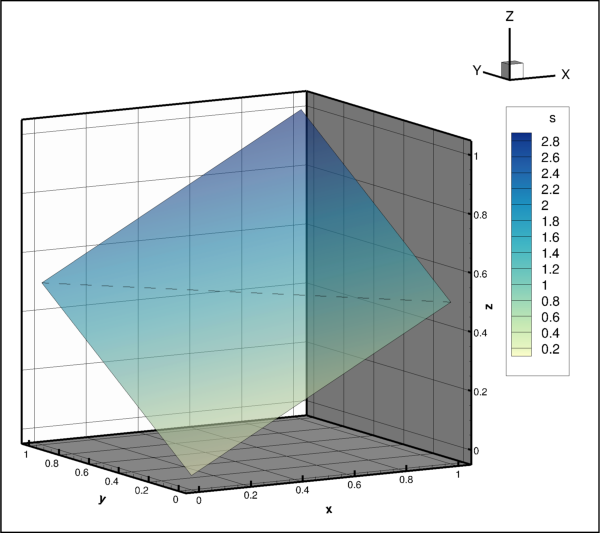
Two triangle polygons showing edge and mesh lines.
Attributes
The data type of the element indices.
The data type of the node indices.
The number of unique nodes in this
Facemap.Methods
alloc(face_nodes[, boundary_faces, ...])Allocate space for the facemap.
Context manager for assigning facemap connections.
boundary_connection(face, offset[, element])The connected element and zone along a boundary face.
face(element, offset)Face index on a specific element.
left_element(face[, element])The element to the left of a specific face.
node(face, offset[, element])The node index along a specific face.
num_boundary_connections([face, element])The number of boundary connections for a given face.
num_faces([element])The number of faces of an element in this
Facemap.num_nodes([face, element])The number nodes for a given face in this
Facemap.right_element(face[, element])The element to the right of a specific face.
set_boundary_connections(elements, zones)Set the boundary connections.
set_elementmap(elementmap)Define connectivity per element.
set_elements(left_elements, right_elements)Sets the polytope connectivity.
set_mapping(facemap, elements[, ...])Set the node and element connectivity for this polytope zone.
set_nodes(facemap)Sets the polytope connectivity.
- Facemap.alloc(face_nodes, boundary_faces=0, boundary_connections=0)[source]
Allocate space for the facemap.
- Parameters:
face_nodes (
int) – Total number of nodes for all faces. This is not the number of unique nodes but the total number. For example if a facemap defines two triangle polygons that share a common face,faceswould be 5 andface_nodeswould be 6, not 4.boundary_faces (
int, optional) – Total number of boundary faces. (default: 0)boundary_connections (
int, optional) – Total number of boundary face elements or boundary face element/zone pairs. (default: 0)
- Returns:
This is called when using the
Facemap.set_mapping()method which is the preferred method for filling the connectivity of polytope zones. If the zone does not already have space allocated for a facemap and if you wish to use theFacemap.set_nodes()andFacemap.set_elements()methods to fill in the connectivity, then this must be called first:>>> facemap = zone.facemap.alloc(400, 25, 50)
Note
Tecplot version 2017.2 or later.
Setting the boundary faces and boundary connections using PyTecplot requires Tecplot version 2017.2 or later.
- Facemap.assignment()[source]
Context manager for assigning facemap connections.
This context ensures the proper book keeping is done when setting the connectivity list and must be used with
Facemap.set_nodes(),Facemap.set_elements()andFacemap.set_boundary_connections(), which are used to define the connectivity of the zone.
- Facemap.boundary_connection(face, offset, element=None)[source]
The connected element and zone along a boundary face.
- Parameters:
- Returns:
-
(element, zone):elementThe zero-based index of the neighboring element.
zoneThe zone holding the neighboring element.
Example usage:
>>> bconn = zone.facemap.boundary_connection(0, 2)
>>> print(bconn.element)
128
>>> print(bconn.zone.index)
2
- Facemap.element_c_type
The data type of the element indices.
Possible values:
ctypes.c_int32,ctypes.c_int64Note
This property is read-only.
- Facemap.face(element, offset)[source]
Face index on a specific element.
- Parameters:
- Returns:
intZero-based index of the face at the specified location.
Example usage:
>>> print(zone.facemap.face(0, 2))
128
- Facemap.left_element(face, element=None)[source]
The element to the left of a specific face.
- Parameters:
- Returns:
A negative number indicates there is no element to the left of this face. Example usage:
>>> print(zone.facemap.left_element(0))
128
- Facemap.node(face, offset, element=None)[source]
The node index along a specific face.
- Parameters:
- Returns:
intThe node at the specified location.
Example usage:
>>> print(zone.facemap.face_node(0, 2))
128
- Facemap.node_c_type
The data type of the node indices.
Possible values:
ctypes.c_int32,ctypes.c_int64Note
This property is read-only.
- Facemap.num_boundary_connections(face=None, element=None)[source]
The number of boundary connections for a given face.
- Parameters:
- Returns:
intThe number of boundary connections.
Example usage:
>>> print(zone.facemap.num_boundary_connections(1))
1
- Facemap.num_faces(element=None)[source]
The number of faces of an element in this
Facemap.- Parameters:
element (
int, optional) – Zero-based index of an element. If no element is given, the total number of faces in the map are returned.- Returns:
Example usage:
>>> print(zone.facemap.num_faces())
1048576
- Facemap.num_nodes(face=None, element=None)[source]
The number nodes for a given face in this
Facemap.- Parameters:
face (
int, required if no element is given) – The zero-based index of the face either within the given element or globally. If no face is given, the number of nodes on the given element are returned.element (
int, required if no face is given) – The zero-based index of an element. If no element is given, then face is globally indexed from zero over the whole zone.
- Returns:
intThe number of nodes.
Example usage:
>>> print(zone.facemap.num_nodes(face=1))
4
- Facemap.num_unique_nodes
The number of unique nodes in this
Facemap.Note
This property is read-only.
Example usage:
>>> print(zone.facemap.num_unique_nodes)
4194304
- Type:
- Facemap.right_element(face, element=None)[source]
The element to the right of a specific face.
- Parameters:
- Returns:
A negative number indicates there is no element to the right of this face. Example usage:
>>> print(zone.facemap.right_element(0))
-1
- Facemap.set_boundary_connections(elements, zones)[source]
Set the boundary connections.
- Parameters:
elements (2D array of
integers) – Zero-based indices of the connected elements. This is a “ragged” array of dimension \((N,E_i)\) where \(N\) is the number of boundary faces and \(E_i\) is the number of boundary connected elements for the \(i^{th}\) face.zones (2D array of
integers) – Zero-based indices of the zones for each entry given in elements. This must be the same shape as elements.
The facemap must first be allocated with
Facemap.alloc()and must be called from within aFacemap.assignment()context, and should follow calls toFacemap.set_nodes()andFacemap.set_elements()to complete the connectivity map information needed for rendering. UsingFacemap.set_mapping()is recommended, which does all the required book keeping.
- Facemap.set_elementmap(elementmap)[source]
Define connectivity per element.
- Parameters:
elementmap (
integers) – Zero-based indices of the nodes that make up each face of each element. For polygons, the map is a list of elements, each made of up a list of nodes. For polyhedrons, this is a list of elements, made up a list of faces, each made up of a list of nodes.
Warning
This method is mutually exclusive with the
Facemap.set_mapping()andFacemap.assignment(),Facemap.set_nodes(),Facemap.set_elements()andFacemap.set_boundary_connections()family of methods. The size of the underlying arrays are calculated based on the elementmap given and a call toFacemap.alloc()is made which will override any previous allocation.This may be a more convenient way to describe the connectivity of a polytope zone, however it does not support boundary face connections to other zones (see
Facemap.set_mapping()).Here is an example of an elementmap for two triangles (polygons):
nodes = ((0, 0, 0  ),
         (1, 0, 0.5),
         (0, 1, 0.5),
         (1, 1, 1  ))
elementmap = ((0, 1, 2),  # polygon 0, 3 faces
              (1, 3, 2))  # polygon 1, 3 faces
This is an example of an elementmap for two tetrahedrons (polyhedrons):
nodes = ((0, 0, 0),
         (1, 1, 0),
         (1, 0, 1),
         (0, 1, 1),
         (0, 0, 1))
elementmap = (((0, 1, 2),  # polyhedron 0, 4 faces
               (0, 1, 3),
               (1, 3, 2),
               (0, 2, 3)),
              ((0, 2, 3),  # polyhedron 1, 4 faces
               (2, 3, 4),
               (0, 2, 4),
               (0, 4, 3)))
- Facemap.set_elements(left_elements, right_elements)[source]
Sets the polytope connectivity.
- Parameters:
The facemap must first be allocated with
Facemap.alloc()and must be called from within aFacemap.assignment()context and should follow a call toFacemap.set_nodes()to complete the connectivity map information needed for rendering. UsingFacemap.set_mapping()is recommended, which does all the required book keeping.
- Facemap.set_mapping(facemap, elements, boundary_elements=None, boundary_zones=None)[source]
Set the node and element connectivity for this polytope zone.
- Parameters:
facemap (2D array of zero-based
integers) – Thelistoflistswhich need not all be the same length, defining the individual elements by their nodes.elements (2D array of zero-based
integers) – This is a \((2,N)\) array where \(N\) is the number of faces and the items are a list of the elements to the left and right of the face respectively.boundary_elements (2D array of
integers, optional) – Zero-based indices of the connected elements. This is a “ragged” array of dimension \((N, E_i)\) where \(N\) is the number of boundary faces and \(E_i\) is the number of boundary connected elements for the \(i^{th}\) face.boundary_zones (2D array of
integers, optional) – Zero-based indices of the zones for each entry given in elements. This must be the same shape as elements.
See the code example for the
Facemapclass object for details.Note
boundary_elements and boundary_zones
The two parameters, boundary_elements and boundary_zones, must be supplied together or not at all.
- Facemap.set_nodes(facemap)[source]
Sets the polytope connectivity.
- Parameters:
facemap (2D array of zero-based
integers) – Thelistoflistswhich need not all be the same length, defining the individual elements by their nodes.
The facemap must first be allocated with
Facemap.alloc()and must be called from within aFacemap.assignment()context and should be followed by a call toFacemap.set_elements()to complete the connectivity map information needed for rendering. It is recomended to use theFacemap.set_mapping()which does all the required book keeping.
FaceNeighbors
- class tecplot.data.FaceNeighbors(zone)[source]
Face neighbor definition and control.
Face neighbors are used when the face of an element overlaps with another face from another element. Specifying these two (or more) overlapping faces as “face neighbors” indicates element connections outside the implicit faces of the nodemap. By specifying face neighbors it ensures that plot elements like shading, creases and edges are treated continously even if there is a zone or cell boundry.
The neighbors can be completely “local”, within a single zone, or “global” conntecting two or more zones together. Furthermore, the connections made can be one-to-one meaning there any given face can only neighbor one other face, or one-to-many where a single face can neighbor several other faces.
This example creates two triangles in two different zones. Global one-to-one face neighbors are then used to stitch the two triangles into a quad. The data created looks like this:
Node positions (x,y,z):

               (1,1,1)
              *
             / \
            /   \
 (0,1,.5)  *-----*  (1,0,.5)
            \   /
             \ /
              *
               (0,0,0)
The two triangles will have separate nodes at the shared locations:
Nodes:
                   2
    Zone 1:       / \
                 /   \
                1-----0
                2-----1
                 \   /
    Zone 0:       \ /
                   0
import tecplot as tp from tecplot.constant import * # Triangle 0 nodes0 = ( (0, 0, 0 ), (1, 0, 0.5), (0, 1, 0.5)) scalar_data0 = (0, 1, 2) conn0 = ((0, 1, 2),) neighbors0 = ((None, 0, None),) neighbor_zones0 = ((None, 1, None),) # Triangle 1 nodes1 = ( (1, 0, 0.5), (0, 1, 0.5), (1, 1, 1 )) scalar_data1 = (1, 2, 3) conn1 = ((0, 1, 2),) neighbors1 = ((0, None, None),) neighbor_zones1 = ((0, None, None),) # Create the dataset and zones ds = tp.active_frame().create_dataset('Data', ['x','y','z','s']) z0 = ds.add_fe_zone(ZoneType.FETriangle, name='FE Triangle Float (3,1) Nodal 0', num_points=len(nodes0), num_elements=len(conn0), face_neighbor_mode=FaceNeighborMode.GlobalOneToOne) z1 = ds.add_fe_zone(ZoneType.FETriangle, name='FE Triangle Float (3,1) Nodal 1', num_points=len(nodes1), num_elements=len(conn1), face_neighbor_mode=FaceNeighborMode.GlobalOneToOne) # Fill in and connect first triangle z0.values('x')[:] = [n[0] for n in nodes0] z0.values('y')[:] = [n[1] for n in nodes0] z0.values('z')[:] = [n[2] for n in nodes0] z0.nodemap[:] = conn0 z0.values('s')[:] = scalar_data0 # Fill in and connect second triangle z1.values('x')[:] = [n[0] for n in nodes1] z1.values('y')[:] = [n[1] for n in nodes1] z1.values('z')[:] = [n[2] for n in nodes1] z1.nodemap[:] = conn1 z1.values('s')[:] = scalar_data1 # Set face neighbors z0.face_neighbors.set_neighbors(neighbors0, neighbor_zones0, obscures=True) z1.face_neighbors.set_neighbors(neighbors1, neighbor_zones1, obscures=True) ### Setup a view of the data plot = tp.active_frame().plot(PlotType.Cartesian3D) plot.activate() plot.contour(0).colormap_name = 'Sequential - Yellow/Green/Blue' plot.contour(0).colormap_filter.distribution = ColorMapDistribution.Continuous for ax in plot.axes: ax.show = True plot.show_mesh = False plot.show_contour = True plot.show_edge = True plot.use_translucency = True # View parameters obtained interactively from Tecplot 360 plot.view.distance = 10 plot.view.width = 2 plot.view.psi = 80 plot.view.theta = 30 plot.view.alpha = 0 plot.view.position = (-4.2, -8.0, 2.3) fmaps = plot.fieldmaps() fmaps.surfaces.surfaces_to_plot = SurfacesToPlot.All fmaps.effects.surface_translucency = 40 # Turning on mesh, we can see all the individual triangles plot.show_mesh = True fmaps.mesh.line_pattern = LinePattern.Dashed plot.contour(0).levels.reset_to_nice() tp.export.save_png('fe_triangles1.png', 600, supersample=3)
Two triangles in two separate zones, stitched together using global face neighbors, showing the edge and mesh.
Attributes
Underlying storage type used by the Tecplot Engine.
Relative locality of the face neighbors.
Methods
add_local_neighbors(neighbors[, offset])Assign all local one-to-one face neighbors at once.
add_neighbors(element, face, neighbors[, ...])Connect boundary of an element's face to a neighboring face.
Context manager for assigning face neighbors.
is_obscured(element, face[, active_zones])Obscuration of the specified face.
neighbors(element, face)Get the neighboring elements and zones of a specific face.
set_neighbors(neighbors[, zones, obscures])Clear and set face neighbors from the given array.
- FaceNeighbors.add_local_neighbors(neighbors, offset=0)[source]
Assign all local one-to-one face neighbors at once.
- Parameters:
This method must be called from within a
FaceNeighbors.assignment()context which will clear any previously existing face neighbor data:>>> with zone.face_neighbors.assigment(): ... zone.face_neighbors.add_local_neighbors(neighbors)
See the example code for
FaceNeighborsclass object for more details on how to set up user-defined face neighbors.
- FaceNeighbors.add_neighbors(element, face, neighbors, zones=None, obscure=False)[source]
Connect boundary of an element’s face to a neighboring face.
This sets the boundary connection face neighbors within an open face neighbor assignment sequence for the specified element and face.
- Parameters:
element (
int) – The element number (zero-based).face (
int) – The face number on the element (zero-based).neighbors (
listofintegersorNone) – List of zero-based indices of the neighboring faces.zones (
listof zone objects, optional) – List of zones for global neighbors. This must be the same length asneighbors. UseNoneto indicate these are local neighbors. (default:None)obscure (
bool, optional) – Indicates that the neighbors completely obscure the face. (default:False)
This method must be called from within a
FaceNeighbors.assignment()context which will clear any previously existing face neighbor data:>>> with zone.face_neighbors.assigment(): ... for elem, face, neighbors, zn in face_neighbor_data: ... zone.face_neighbors.add_neighbors(elem, face, ... neighbors, zn)
See the example code for
FaceNeighborsclass object for more details on how to set up user-defined face neighbors.
- FaceNeighbors.assignment()[source]
Context manager for assigning face neighbors.
This context ensures the proper book keeping is done when setting face neighbors. After the face neighbors are specified, this context will valid the connections and make appropriate changes to the zone metadata. It must be used with the
FaceNeighbors.add_local_neighbors()and/orFaceNeighbors.add_neighbors()methods. See theFaceNeighborsexample code for more details on how to set up user-defined face neighbors.
- FaceNeighbors.c_type
Underlying storage type used by the Tecplot Engine.
Possible values:
ctypes.c_int32, ctypes.c_int64`.Note
This property is read-only.
- FaceNeighbors.is_obscured(element, face, active_zones=None)[source]
Obscuration of the specified face.
- Parameters:
- Returns:
Note
Because datasets can be shared between frames, the default frame used to identify the active zones may not be the one you want. In this case, you can use the
Frame.active_zones()method to provide the active zones for a specific frame. Furthermore, the plot type of the frame must have the concept of active zones - i.e. it must not be in “sketch” mode.Example usage:
>>> zone.face_neighbors.is_obscured(element=0, face=1)
True
- FaceNeighbors.mode
Relative locality of the face neighbors.
- Possible values:
FaceNeighborMode.LocalOneToOne, FaceNeighborMode.LocalOneToMany,FaceNeighborMode.GlobalOneToOne,FaceNeighborMode.GlobalOneToMany.
Note
This property is read-only.
Face neighbors are used when the face of an element overlaps with another face from another element. The neighbors can be completely “local”, within a single zone, or “global” conntecting two or more zones together. Furthermore, the connections made can be one-to-one meaning there any given face can only neighbor one other face, or one-to-many where a single face can neighbor several other faces. The face neighbor mode is set on zone creation and can not be changed afterwards:
>>> zone = dataset.add_fe_zone(ZoneType.FETriangle, 'Zone', 4, 2,
...    face_neighbor_mode=FaceNeighborMode.LocalOneToMany)
>>> print(zone.face_neighbors.mode)
FaceNeighborMode.LocalOneToMany
- Type:
- Possible values:
- FaceNeighbors.neighbors(element, face)[source]
Get the neighboring elements and zones of a specific face.
- Parameters:
- Returns:
listofnamedtuples–(element, zone):element:The zero-based index of the neighboring element.
zone:The zone holding the neighboring element. A value of
Noneindicates this is a local (intra-zone) neighbor connection.
Example getting the neighboring faces of a zone’s first element, second face:
>>> neighbors = zone.face_neighbors.neighbors(element=0, face=1)
>>> for neighbor in neighbors:
...     elem, zn = neighbor
...     print(elem, zn.index)
21 2
- FaceNeighbors.set_neighbors(neighbors, zones=None, obscures=False)[source]
Clear and set face neighbors from the given array.
- Parameters:
neighbors (array of
integers) – Zero-based Element indices of the neighbors for each face in the zone. A value of \(-1\) orNoneindicates no neighbor.zones (array of Zones, optional) – This parameter is only used when the face neighbor mode is global one-to-one or global one-to-many. (default:
None)obscures (array of
booleans, optional) – Indicates that the neighbors completely obscure the face. (default:False)
This method uses the
FaceNeighbors.assignment()context internally to ensure the proper book keeping is done. See the example code forFaceNeighborsclass object for details on how to use this method.
Auxiliary Data
AuxData
- class tecplot.session.AuxData(parent, object_type, object_index=None)[source]
Auxiliary data.
The Tecplot Engine can hold auxiliary data attached to one of the following objects:
Auxiliary data is an ordered key-value pair that behaves like an ordered dictionary, or
OrderedDict. Keys are strings which are ordered alphabetically and values can additionally be access by index. The keys must be alphanumeric (special characters “.” and “_” are allowed), must not contain spaces, and must begin with a non-numeric character or underscore. Values, on the other hand, are arbitrary strings and can contain anything except the null character. In this example, we query the auxiliary data attached to the dataset and add some information to it. Notice that the stored order is alphabetical:import tecplot as tp aux = tp.active_frame().aux_data aux['info'] = 'Here is some information.' aux['Xavg'] = 3.14159 aux['note'] = 'Aux data values are always converted to strings.' ''' The following code will print: info: Here is some information. note: Aux data values are always converted to strings. Xavg: 3.14159 ''' for k, v in aux.items(): print('{}: {}'.format(k,v))
Methods
as_dict()Returns a Python dict of the Aux Data attached to the parent.
clear()Deletes all Aux Data from the associated object.
index(key)Returns the zero-based index of the element based on key.
items()Yields all key/value pairs of the Aux Data attached to the parent.
key(index)Returns the key at a specific zero-based index.
keys()Yields all keys of the Aux Data attached to the parent.
update(*other, **kwargs)Update Aux Data with key/value pairs from another Aux Data or dict.
values()Yields all values of the Aux Data attached to the parent.
- AuxData.as_dict()[source]
Returns a Python dict of the Aux Data attached to the parent.
Note that this will remove the alphabetical ordering guarantee that Aux Data has since Python dict objects are unordered. Example usage:
>>> frame = tp.active_frame()
>>> frame.aux_data['result'] = '3.1415'
>>> frame.aux_data['other_info'] = '128'
>>> aux = frame.aux_data.as_dict()
>>> print(aux)
{'result': '3.1415', 'other_info': '128'}
- AuxData.clear()[source]
Deletes all Aux Data from the associated object.
Example usage:
>>> print(frame.aux_data)
{'bb': 'test bb', 'cc': 'test cc', 'aa': 'test aa'}
>>> frame.aux_data.clear()
>>> print(frame.aux_data)
{}
- AuxData.index(key)[source]
Returns the zero-based index of the element based on key.
Example usage:
>>> frame = tp.active_frame()
>>> frame.aux_data['result'] = '3.1415'
>>> frame.aux_data['other_info'] = '128'
>>> print(frame.aux_data.index('other_info'))
0
>>> print(frame.aux_data.index('result'))
1
- AuxData.items()[source]
Yields all key/value pairs of the Aux Data attached to the parent.
Elements are always ordered alphabetically by the keys. Example usage:
>>> frame = tp.active_frame()
>>> frame.aux_data['result'] = '3.1415'
>>> frame.aux_data['other_info'] = '128'
>>> for key, value in frame.aux_data.items():
...     print(key, value)
other_info 128
result 3.1415
- AuxData.key(index)[source]
Returns the key at a specific zero-based index.
Example usage:
>>> frame = tp.active_frame()
>>> frame.aux_data['result'] = '3.1415'
>>> frame.aux_data['other_info'] = '128'
>>> print(frame.aux_data.key(0))
other_info
>>> print(frame.aux_data.key(1))
result
- AuxData.keys()[source]
Yields all keys of the Aux Data attached to the parent.
Elements are always ordered alphabetically by the keys. Example usage:
>>> frame = tp.active_frame()
>>> frame.aux_data['result'] = '3.1415'
>>> frame.aux_data['other_info'] = '128'
>>> for value in frame.aux_data.keys():
...     print(value)
other_info
result
- AuxData.update(*other, **kwargs)[source]
Update Aux Data with key/value pairs from another Aux Data or dict.
Example usage:
>>> frame = tp.active_frame()
>>> frame.aux_data.update({'result': '3.1415', 'other_info': '128'})
>>> print(frame.aux_data)
{'result': '3.1415', 'other_info': '128'}
- AuxData.values()[source]
Yields all values of the Aux Data attached to the parent.
Elements are always ordered alphabetically by the keys. Example usage:
>>> frame = tp.active_frame() >>> frame.aux_data['result'] = '3.1415' >>> frame.aux_data['other_info'] = '128' >>> for value in frame.aux_data.values(): ... print(value) 128 3.1415