Plot¶

Plots ¶

Cartesian2DFieldPlot ¶

class tecplot.plot.Cartesian2DFieldPlot(frame)[source]¶

2D plot containing field data associated with style through fieldmaps.

from os import path
import tecplot as tp
from tecplot.constant import PlotType

examples_dir = tp.session.tecplot_examples_directory()
infile = path.join(examples_dir, 'SimpleData', 'HeatExchanger.plt')
dataset = tp.data.load_tecplot(infile)

frame = tp.active_frame()
plot = frame.plot(PlotType.Cartesian2D)
plot.activate()

plot.vector.u_variable = dataset.variable('U(M/S)')
plot.vector.v_variable = dataset.variable('V(M/S)')

plot.contour(2).variable = dataset.variable('T(K)')
plot.contour(2).colormap_name = 'Sequential - Yellow/Green/Blue'

for z in dataset.zones():
    fmap = plot.fieldmap(z)
    fmap.contour.flood_contour_group = plot.contour(2)

plot.show_contour = True
plot.show_vector = True

# ensure consistent output between interactive (connected) and batch
plot.contour(2).levels.reset_to_nice()

# save image to file
tp.export.save_png('plot_field2d.png', 600, supersample=3)

Attributes

`active_fieldmap_indices`	Set of active fieldmaps by index.
`active_fieldmaps`	Active fieldmaps in this plot.
`axes`	Axes style control for this plot.
`data_labels`	Node and cell labels.
`draw_order`	The order in which objects are drawn to the screen.
`hoe_settings`	High order element settings.
`ijk_blanking`	Mask off cells by \((i, j, k)\) index.
`linking_between_frames`	Style linking between frames.
`num_fieldmaps`	Number of all fieldmaps in this plot.
`num_solution_times`	Number of solution times for all active fieldmaps.
`rgb_coloring`	RGB contour flooding style control.
`scatter`	Plot-local `Scatter` style control.
`show_contour`	Enable contours for this plot.
`show_edge`	Enable zone edge lines for this plot.
`show_isosurfaces`	Show isosurfaces for this plot.
`show_mesh`	Enable mesh lines for this plot.
`show_scatter`	Enable scatter symbols for this plot.
`show_shade`	Enable surface shading effect for this plot.
`show_slices`	Show slices for this plot.
`show_streamtraces`	Enable drawing `Streamtraces` on this plot.
`show_vector`	Enable drawing of vectors.
`solution_time`	The current solution time.
`solution_times`	`List` of active solution times.
`solution_timestep`	The zero-based index of the current solution time.
`streamtraces`	Plot-local `streamtrace` attributes.
`transient_zone_visibility`	Policy to determine transient visibility of zones.
`value_blanking`	Mask off cells by value.
`vector`	Vector variable and style control for this plot.
`view`	Axes orientation and limits adjustments.

Methods

`activate`()	Make this the active plot type on the parent frame.
`activated`()	Context to ensure this plot is active.
`contour`(index)	`ContourGroup`: Plot-local `ContourGroup` style control.
`fieldmap`(key)	Returns a `Cartesian2DFieldmap` by Zone or index.
`fieldmap_index`(zone)	The index of the fieldmap associated with a Zone.
`fieldmaps`(*keys)	`Cartesian2DFieldmapCollection` by Zones or indices.

Cartesian2DFieldPlot.activate()[source]¶

Make this the active plot type on the parent frame.

Example usage:

>>> from tecplot.constant import PlotType
>>> plot = frame.plot(PlotType.Cartesian2D)
>>> plot.activate()

Cartesian2DFieldPlot.activated()¶

Context to ensure this plot is active.

Example usage:

>>> from tecplot.constant import PlotType
>>> frame = tecplot.active_frame()
>>> frame.plot_type = PlotType.XYLine  # set active plot type
>>> plot = frame.plot(PlotType.Cartesian3D)  # get inactive plot
>>> print(frame.plot_type)
PlotType.XYLine
>>> with plot.activated():
...     print(frame.plot_type)  # 3D plot temporarily active
PlotType.Cartesian3D
>>> print(frame.plot_type)  # original plot type restored
PlotType.XYLine

Cartesian2DFieldPlot.active_fieldmap_indices¶

Set of active fieldmaps by index.

This example sets the first three fieldmaps active, disabling all others. It then turns on scatter symbols for just these three:

>>> plot.active_fieldmap_indices = [0, 1, 2]
>>> plot.fieldmaps(0, 1, 2).scatter.show = True

Type:: set

Cartesian2DFieldPlot.active_fieldmaps¶

Active fieldmaps in this plot.

Example usage:

>>> plot.active_fieldmaps.vector.show = True

Note

Possible side-effect when connected to Tecplot 360.

Changing the solution times in the dataset or modifying the active fieldmaps in a frame may trigger a change in the active plot’s solution time by the Tecplot 360 interface. This is done to keep the GUI controls consistent. In batch mode, no such side-effect will take place and the user must take care to set the plot’s solution time with the plot.solution_time or plot.solution_timestep properties.

Type:: Cartesian2DFieldmapCollection

Cartesian2DFieldPlot.axes¶

Axes style control for this plot.

Example usage:

>>> from tecplot.constant import PlotType
>>> frame.plot_type = PlotType.Cartesian2D
>>> axes = frame.plot().axes
>>> axes.x_axis.variable = dataset.variable('U')
>>> axes.y_axis.variable = dataset.variable('V')

Type:: Cartesian2DFieldAxes

Cartesian2DFieldPlot.contour(index)¶

ContourGroup: Plot-local ContourGroup style control.

Example usage:

>>> contour = frame.plot().contour(0)
>>> contour.colormap_name = 'Magma'

Cartesian2DFieldPlot.data_labels¶

Node and cell labels.

This object controls displaying labels for every node and/or cell in the dataset. Example usage:

>>> plot.data_labels.show_cell_labels = True
>>> plot.data_labels.step_index = 10

Type:: FieldPlotDataLabels

Cartesian2DFieldPlot.draw_order¶

The order in which objects are drawn to the screen.

Possible values: TwoDDrawOrder.ByZone, TwoDDrawOrder.ByLayer.

The order is either by Zone or by visual layer (contour, mesh, etc.):

>>> plot.draw_order = TwoDDrawOrder.ByZone

Type:: TwoDDrawOrder

Cartesian2DFieldPlot.fieldmap(key)[source]¶

Returns a Cartesian2DFieldmap by Zone or index.

Parameters:: key (Zone or int) – The Zone must be in the Dataset attached to the associated frame of this plot. A negative index is interpreted as counting from the end of the available fieldmaps.

Example usage:

>>> fmap = plot.fieldmap(dataset.zone(0))
>>> fmap.scatter.show = True

Cartesian2DFieldPlot.fieldmap_index(zone)¶

The index of the fieldmap associated with a Zone.

Parameters:: zone (Zone) – The Zone object that belongs to the Dataset associated with this plot.
Returns:: Index

Example usage:

>>> fmap_index = plot.fieldmap_index(dataset.zone('Zone'))
>>> plot.fieldmap(fmap_index).show_mesh = True

Cartesian2DFieldPlot.fieldmaps(*keys)[source]¶

Cartesian2DFieldmapCollection by Zones or indices.

Parameters:: keys (list of Zones or ints) – The Zones must be in the Dataset attached to the associated frame of this plot. Negative indices are interpreted as counting from the end of the available fieldmaps.

Example usage:

>>> fmaps = plot.fieldmaps(dataset.zone(0), dataset.zone(1))
>>> fmaps.scatter.show = True

Changed in version 0.9: fieldmaps was changed from a property (0.8 and earlier) to a method requiring parentheses.

Cartesian2DFieldPlot.hoe_settings¶

High order element settings.

Example usage:

>>> plot.hoe_settings.num_subdivision_levels = 3

Type:: FieldPlotHOESettings

Cartesian2DFieldPlot.ijk_blanking¶

Mask off cells by \((i, j, k)\) index.

Example usage:

>>> plot.ijk_blanking.min_percent = (50, 50)
>>> plot.ijk_blanking.active = True

Type:: IJKBlanking

Cartesian2DFieldPlot.linking_between_frames¶

Style linking between frames.

Example usage:

>>> plot.linking_between_frames.group = 1
>>> plot.linking_between_frames.link_solution_time = True

Type:: Cartesian2DPlotLinkingBetweenFrames

Cartesian2DFieldPlot.num_fieldmaps¶

Number of all fieldmaps in this plot.

Example usage:

>>> print(frame.plot().num_fieldmaps)
3

Type:: int

Cartesian2DFieldPlot.num_solution_times¶

Number of solution times for all active fieldmaps.

Note

This only returns the number of active solution times. When assigning strands and solution times to zones, the zones are placed into an inactive fieldmap that must be subsequently activated. See example below.

>>> # place all zones into a single fieldmap (strand: 1)
>>> # with incrementing solution times
>>> for time, zone in enumerate(dataset.zones()):
...     zone.strand = 1
...     zone.solution_time = time
...
>>> # We must activate the fieldmap to ensure the plot's
>>> # solution times have been updated. Since we placed
>>> # all zones into a single fieldmap, we can assume the
>>> # first fieldmap (index: 0) is the one we want.
>>> plot.active_fieldmaps += [0]
>>>
>>> # now the plot's solution times are available.
>>> print(plot.num_solution_times)
10
>>> print(plot.solution_times)
[0.0, 1.0, 2.0, 3.0, 4.0, 5.0, 6.0, 7.0, 8.0, 9.0]

New in version 2017.2: Solution time manipulation requires Tecplot 360 2017 R2 or later.

Type:: int

Cartesian2DFieldPlot.rgb_coloring¶

RGB contour flooding style control.

Example usage:

>>> plot.rgb_coloring.red_variable = dataset.variable('gas')
>>> plot.rgb_coloring.green_variable = dataset.variable('oil')
>>> plot.rgb_coloring.blue_variable = dataset.variable('water')
>>> plot.show_contour = True
>>> plot.fieldmaps().contour.flood_contour_group = plot.rgb_coloring

Type:: RGBColoring

Cartesian2DFieldPlot.scatter¶

Plot-local Scatter style control.

Example usage:

>>> scatter = frame.plot().scatter
>>> scatter.variable = dataset.variable('P')

Type:: Scatter

Cartesian2DFieldPlot.show_contour¶

Enable contours for this plot.

Example usage:

>>> frame.plot().show_contour = True

Type:: bool

Cartesian2DFieldPlot.show_edge¶

Enable zone edge lines for this plot.

Example usage:

>>> frame.plot().show_edge = True

Type:: bool

Cartesian2DFieldPlot.show_isosurfaces¶

Show isosurfaces for this plot.

Example usage:

>>> frame.plot().show_isosurfaces(True)

Type:: bool

Cartesian2DFieldPlot.show_mesh¶

Enable mesh lines for this plot.

Example usage:

>>> frame.plot().show_mesh = True

Type:: bool

Cartesian2DFieldPlot.show_scatter¶

Enable scatter symbols for this plot.

Example usage:

>>> frame.plot().show_scatter = True

Type:: bool

Cartesian2DFieldPlot.show_shade¶

Enable surface shading effect for this plot.

Example usage:

>>> frame.plot().show_shade = True

Type:: bool

Cartesian2DFieldPlot.show_slices¶

Show slices for this plot.

Example usage:

>>> frame.plot().show_slices(True)

Type:: bool

Cartesian2DFieldPlot.show_streamtraces¶

Enable drawing Streamtraces on this plot.

Example usage:

>>> frame.plot().show_streamtraces = True

Type:: bool

Cartesian2DFieldPlot.show_vector¶

Enable drawing of vectors.

Example usage:

>>> frame.plot().show_vector = True

Type:: bool

Cartesian2DFieldPlot.solution_time¶

The current solution time.

Example usage:

>>> print(plot.solution_times)
[0.0, 1.0, 2.0]
>>> plot.solution_time = 1.0

Note

Possible side-effect when connected to Tecplot 360.

Changing the solution times in the dataset or modifying the active fieldmaps in a frame may trigger a change in the active plot’s solution time by the Tecplot 360 interface. This is done to keep the GUI controls consistent. In batch mode, no such side-effect will take place and the user must take care to set the plot’s solution time with the plot.solution_time or plot.solution_timestep properties.

New in version 2017.2: Solution time manipulation requires Tecplot 360 2017 R2 or later.

Type:: float

Cartesian2DFieldPlot.solution_times¶

List of active solution times.

Note

This only returns the list of active solution times. When assigning strands and solution times to zones, the zones are placed into an inactive fieldmap that must be subsequently activated. See example below.

Example usage:

>>> print(plot.solution_times)
[0.0, 1.0, 2.0]

New in version 2017.2: Solution time manipulation requires Tecplot 360 2017 R2 or later.

Type:: list of floats

Cartesian2DFieldPlot.solution_timestep¶

The zero-based index of the current solution time.

A negative index is interpreted as counting from the end of the available solution timesteps. Example usage:

>>> print(plot.solution_times)
[0.0, 1.0, 2.0]
>>> print(plot.solution_time)
0.0
>>> plot.solution_timestep += 1
>>> print(plot.solution_time)
1.0

Note

Possible side-effect when connected to Tecplot 360.

Changing the solution times in the dataset or modifying the active fieldmaps in a frame may trigger a change in the active plot’s solution time by the Tecplot 360 interface. This is done to keep the GUI controls consistent. In batch mode, no such side-effect will take place and the user must take care to set the plot’s solution time with the plot.solution_time or plot.solution_timestep properties.

New in version 2017.2: Solution time manipulation requires Tecplot 360 2017 R2 or later.

Type:: int

Cartesian2DFieldPlot.streamtraces¶

Plot-local streamtrace attributes.

Example usage:

>>> streamtraces = frame.plot().streamtraces
>>> streamtraces.color = Color.Blue

Type:: Streamtraces

Cartesian2DFieldPlot.transient_zone_visibility¶

Policy to determine transient visibility of zones.

Possible values: ZonesAtOrBeforeSolutionTime, ZonesAtSolutionTime.

Example usage:

>>> from tecplot.constant import TransientZoneVisibility
>>> plot.transient_zone_visibility = \
...     TransientZoneVisibility.ZonesAtSolutionTime

New in version 2021.2: Transient zone visibility requires Tecplot 360 2021 R2 or later.

Type:: TransientZoneVisibility

Cartesian2DFieldPlot.value_blanking¶

Mask off cells by value.

Example usage:

>>> plot.value_blanking.constraint(0).comparison_value = 3.14
>>> plot.value_blanking.constraint(0).active = True

Type:: ValueBlanking

Cartesian2DFieldPlot.vector¶

Vector variable and style control for this plot.

Example usage:

>>> plot.vector.u_variable = dataset.variable('U')

Type:: Vector2D

Cartesian2DFieldPlot.view¶

Axes orientation and limits adjustments.

Example usage:

>>> plot.view.fit()

Type:: Cartesian2DFieldView

Cartesian3DFieldPlot ¶

class tecplot.plot.Cartesian3DFieldPlot(frame)[source]¶

3D plot containing field data associated with style through fieldmaps.

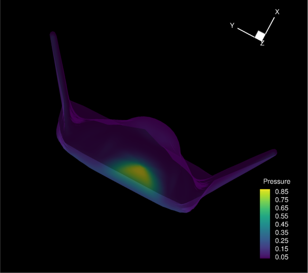
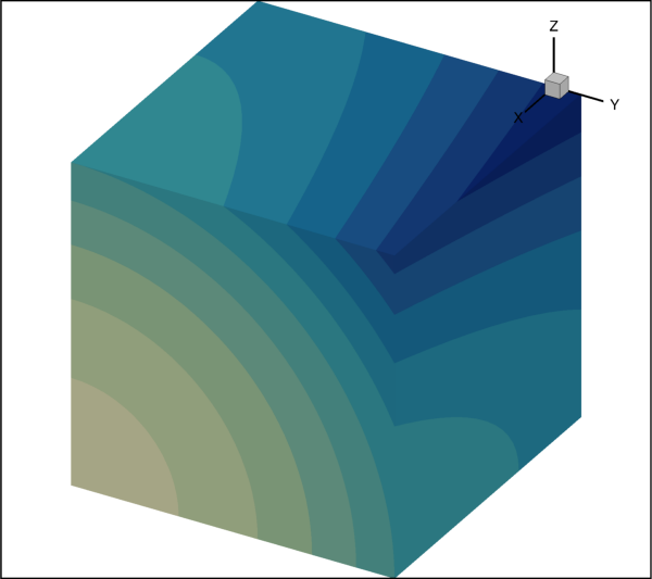
from os import path
import tecplot as tp
from tecplot.constant import PlotType

examples_dir = tp.session.tecplot_examples_directory()
infile = path.join(examples_dir, 'SimpleData', 'SpaceShip.lpk')
dataset = tp.load_layout(infile)

frame = tp.active_frame()
plot = frame.plot(PlotType.Cartesian3D)
plot.activate()
plot.use_lighting_effect = False
plot.show_streamtraces = False
plot.use_translucency = True

# ensure consistent output between interactive (connected) and batch
plot.contour(0).levels.reset_to_nice()

# save image to file
tp.export.save_png('plot_field3d.png', 600, supersample=3)

Attributes

`active_fieldmap_indices`	Set of active fieldmaps by index.
`active_fieldmaps`	Active fieldmaps in this plot.
`axes`	Axes style control for this plot.
`data_labels`	Node and cell labels.
`hoe_settings`	High order element settings.
`ijk_blanking`	Mask off cells by \((i, j, k)\) index.
`light_source`	Control the direction and effects of lighting.
`line_lift_fraction`	Lift lines above plot by percentage distance to the eye.
`linking_between_frames`	Style linking between frames.
`near_plane_fraction`	position of the "near plane".
`num_fieldmaps`	Number of all fieldmaps in this plot.
`num_solution_times`	Number of solution times for all active fieldmaps.
`perform_extra_sorting`	Use a more robust depth sorting algorithm for display.
`rgb_coloring`	RGB contour flooding style control.
`scatter`	Plot-local `Scatter` style control.
`show_contour`	Enable contours for this plot.
`show_edge`	Enable zone edge lines for this plot.
`show_isosurfaces`	Show isosurfaces for this plot.
`show_mesh`	Enable mesh lines for this plot.
`show_scatter`	Enable scatter symbols for this plot.
`show_shade`	Enable surface shading effect for this plot.
`show_slices`	Show slices for this plot.
`show_streamtraces`	Enable drawing `Streamtraces` on this plot.
`show_vector`	Enable drawing of vectors.
`solution_time`	The current solution time.
`solution_times`	`List` of active solution times.
`solution_timestep`	The zero-based index of the current solution time.
`streamtraces`	Plot-local `streamtrace` attributes.
`symbol_lift_fraction`	Lift symbols above plot by percentage distance to the eye.
`transient_zone_visibility`	Policy to determine transient visibility of zones.
`use_lighting_effect`	Enable lighting effect for all objects within this plot.
`use_translucency`	Enable translucent effect for all objects within this plot.
`value_blanking`	Mask off cells by value.
`vector`	Vector variable and style control for this plot.
`vector_lift_fraction`	Lift vectors above plot by percentage distance to the eye.
`view`	Viewport, axes orientation and limits adjustments.

Methods

`activate`()	Make this the active plot type on the parent frame.
`activated`()	Context to ensure this plot is active.
`contour`(index)	`ContourGroup`: Plot-local `ContourGroup` style control.
`fieldmap`(key)	Returns a `Cartesian3DFieldmap` by Zone or index.
`fieldmap_index`(zone)	The index of the fieldmap associated with a Zone.
`fieldmaps`(*keys)	`Cartesian3DFieldmapCollection` by Zones or indices.
`isosurface`(index)	`IsosurfaceGroup`: Plot-local `isosurface` settings.
`slice`(index)	`SliceGroup`: Plot-local `slice` style control.
`slices`(*indices)	`SliceGroupCollection`: Plot-local slice style control.

Cartesian3DFieldPlot.activate()[source]¶

Make this the active plot type on the parent frame.

Example usage:

>>> from tecplot.constant import PlotType
>>> plot = frame.plot(PlotType.Cartesian3D)
>>> plot.activate()

Cartesian3DFieldPlot.activated()¶

Context to ensure this plot is active.

Example usage:

>>> from tecplot.constant import PlotType
>>> frame = tecplot.active_frame()
>>> frame.plot_type = PlotType.XYLine  # set active plot type
>>> plot = frame.plot(PlotType.Cartesian3D)  # get inactive plot
>>> print(frame.plot_type)
PlotType.XYLine
>>> with plot.activated():
...     print(frame.plot_type)  # 3D plot temporarily active
PlotType.Cartesian3D
>>> print(frame.plot_type)  # original plot type restored
PlotType.XYLine

Cartesian3DFieldPlot.active_fieldmap_indices¶

Set of active fieldmaps by index.

This example sets the first three fieldmaps active, disabling all others. It then turns on scatter symbols for just these three:

>>> plot.active_fieldmap_indices = [0, 1, 2]
>>> plot.fieldmaps(0, 1, 2).scatter.show = True

Type:: set

Cartesian3DFieldPlot.active_fieldmaps¶

Active fieldmaps in this plot.

Example usage:

>>> plot.active_fieldmaps.vector.show = True

Note

Possible side-effect when connected to Tecplot 360.

Changing the solution times in the dataset or modifying the active fieldmaps in a frame may trigger a change in the active plot’s solution time by the Tecplot 360 interface. This is done to keep the GUI controls consistent. In batch mode, no such side-effect will take place and the user must take care to set the plot’s solution time with the plot.solution_time or plot.solution_timestep properties.

Type:: Cartesian3DFieldmapCollection

Cartesian3DFieldPlot.axes¶

Axes style control for this plot.

Example usage:

>>> from tecplot.constant import PlotType
>>> frame.plot_type = PlotType.Cartesian3D
>>> axes = frame.plot().axes
>>> axes.x_axis.variable = dataset.variable('U')
>>> axes.y_axis.variable = dataset.variable('V')
>>> axes.z_axis.variable = dataset.variable('W')

Type:: Cartesian3DFieldAxes

Cartesian3DFieldPlot.contour(index)¶

ContourGroup: Plot-local ContourGroup style control.

Example usage:

>>> contour = frame.plot().contour(0)
>>> contour.colormap_name = 'Magma'

Cartesian3DFieldPlot.data_labels¶

Node and cell labels.

This object controls displaying labels for every node and/or cell in the dataset. Example usage:

>>> plot.data_labels.show_cell_labels = True
>>> plot.data_labels.step_index = 10

Type:: FieldPlotDataLabels

Cartesian3DFieldPlot.fieldmap(key)[source]¶

Returns a Cartesian3DFieldmap by Zone or index.

Parameters:: key (Zone or int) – The Zone must be in the Dataset attached to the associated frame of this plot. A negative index is interpreted as counting from the end of the available fieldmaps.

Example usage:

>>> fmap = plot.fieldmap(dataset.zone(0))
>>> fmap.scatter.show = True

Cartesian3DFieldPlot.fieldmap_index(zone)¶

The index of the fieldmap associated with a Zone.

Parameters:: zone (Zone) – The Zone object that belongs to the Dataset associated with this plot.
Returns:: Index

Example usage:

>>> fmap_index = plot.fieldmap_index(dataset.zone('Zone'))
>>> plot.fieldmap(fmap_index).show_mesh = True

Cartesian3DFieldPlot.fieldmaps(*keys)[source]¶

Cartesian3DFieldmapCollection by Zones or indices.

Parameters:: keys (list of Zones or integers) – The Zones must be in the Dataset attached to the associated frame of this plot. Negative indices are interpreted as counting from the end of the available fieldmaps.

Example usage:

>>> fmaps = plot.fieldmaps(dataset.zone(0), dataset.zone(1))
>>> fmaps.scatter.show = True

Changed in version 0.9: fieldmaps was changed from a property (0.8 and earlier) to a method requiring parentheses.

Cartesian3DFieldPlot.hoe_settings¶

High order element settings.

Example usage:

>>> plot.hoe_settings.num_subdivision_levels = 3

Type:: FieldPlotHOESettings

Cartesian3DFieldPlot.ijk_blanking¶

Mask off cells by \((i, j, k)\) index.

Example usage:

>>> plot.ijk_blanking.min_percent = (50, 50)
>>> plot.ijk_blanking.active = True

Type:: IJKBlanking

Cartesian3DFieldPlot.isosurface(index)[source]¶

IsosurfaceGroup: Plot-local isosurface settings.

Example usage:

>>> isosurface_0 = frame.plot().isosurface(0)
>>> isosurface_0.mesh.color = Color.Blue

Cartesian3DFieldPlot.light_source¶

Control the direction and effects of lighting.

Example usage:

>>> plot.light_source.intensity = 70.0

Type:: LightSource

Cartesian3DFieldPlot.line_lift_fraction¶

Lift lines above plot by percentage distance to the eye.

Example usage:

>>> plot.line_lift_fraction = 0.6

Type:: float

Cartesian3DFieldPlot.linking_between_frames¶

Style linking between frames.

Example usage:

>>> plot.linking_between_frames.group = 1
>>> plot.linking_between_frames.link_solution_time = True

Type:: Cartesian3DPlotLinkingBetweenFrames

Cartesian3DFieldPlot.near_plane_fraction¶

position of the “near plane”.

In a 3D plot, the “near plane” acts as a windshield. Anything in front of this plane does not display. Example usage:

>>> plot.near_plane_fraction = 0.1

Type:: float

Cartesian3DFieldPlot.num_fieldmaps¶

Number of all fieldmaps in this plot.

Example usage:

>>> print(frame.plot().num_fieldmaps)
3

Type:: int

Cartesian3DFieldPlot.num_solution_times¶

Number of solution times for all active fieldmaps.

Note

This only returns the number of active solution times. When assigning strands and solution times to zones, the zones are placed into an inactive fieldmap that must be subsequently activated. See example below.

>>> # place all zones into a single fieldmap (strand: 1)
>>> # with incrementing solution times
>>> for time, zone in enumerate(dataset.zones()):
...     zone.strand = 1
...     zone.solution_time = time
...
>>> # We must activate the fieldmap to ensure the plot's
>>> # solution times have been updated. Since we placed
>>> # all zones into a single fieldmap, we can assume the
>>> # first fieldmap (index: 0) is the one we want.
>>> plot.active_fieldmaps += [0]
>>>
>>> # now the plot's solution times are available.
>>> print(plot.num_solution_times)
10
>>> print(plot.solution_times)
[0.0, 1.0, 2.0, 3.0, 4.0, 5.0, 6.0, 7.0, 8.0, 9.0]

New in version 2017.2: Solution time manipulation requires Tecplot 360 2017 R2 or later.

Type:: int

Cartesian3DFieldPlot.perform_extra_sorting¶

Use a more robust depth sorting algorithm for display.

When printing 3D plots in a vector graphics format, Tecplot 360 must sort the objects so that it can draw those farthest from the screen first and those closest to the screen last. By default, Tecplot 360 uses a quick sorting algorithm. This is not always accurate and does not detect problems such as intersecting objects. When perform_extra_sorting set to True, Tecplot 360 uses a slower, more accurate approach that detects and resolves such problems. Example usage:

>>> plot.perform_extra_sorting = True

Type:: bool

Cartesian3DFieldPlot.rgb_coloring¶

RGB contour flooding style control.

Example usage:

>>> plot.rgb_coloring.red_variable = dataset.variable('gas')
>>> plot.rgb_coloring.green_variable = dataset.variable('oil')
>>> plot.rgb_coloring.blue_variable = dataset.variable('water')
>>> plot.show_contour = True
>>> plot.fieldmaps().contour.flood_contour_group = plot.rgb_coloring

Type:: RGBColoring

Cartesian3DFieldPlot.scatter¶

Plot-local Scatter style control.

Example usage:

>>> scatter = frame.plot().scatter
>>> scatter.variable = dataset.variable('P')

Type:: Scatter

Cartesian3DFieldPlot.show_contour¶

Enable contours for this plot.

Example usage:

>>> frame.plot().show_contour = True

Type:: bool

Cartesian3DFieldPlot.show_edge¶

Enable zone edge lines for this plot.

Example usage:

>>> frame.plot().show_edge = True

Type:: bool

Cartesian3DFieldPlot.show_isosurfaces¶

Show isosurfaces for this plot.

Example usage:

>>> frame.plot().show_isosurfaces(True)

Type:: bool

Cartesian3DFieldPlot.show_mesh¶

Enable mesh lines for this plot.

Example usage:

>>> frame.plot().show_mesh = True

Type:: bool

Cartesian3DFieldPlot.show_scatter¶

Enable scatter symbols for this plot.

Example usage:

>>> frame.plot().show_scatter = True

Type:: bool

Cartesian3DFieldPlot.show_shade¶

Enable surface shading effect for this plot.

Example usage:

>>> frame.plot().show_shade = True

Type:: bool

Cartesian3DFieldPlot.show_slices¶

Show slices for this plot.

Example usage:

>>> frame.plot().show_slices(True)

Type:: bool

Cartesian3DFieldPlot.show_streamtraces¶

Enable drawing Streamtraces on this plot.

Example usage:

>>> frame.plot().show_streamtraces = True

Type:: bool

Cartesian3DFieldPlot.show_vector¶

Enable drawing of vectors.

Example usage:

>>> frame.plot().show_vector = True

Type:: bool

Cartesian3DFieldPlot.slice(index)[source]¶

SliceGroup: Plot-local slice style control.

Example usage:

>>> from tecplot.constant import Color
>>> slice0 = frame.plot().slice(0)
>>> slice0.mesh.show = True
>>> slice0.mesh.color = Color.Blue

Cartesian3DFieldPlot.slices(*indices)[source]¶

SliceGroupCollection: Plot-local slice style control.

Example setting setting mesh color of all slices to blue:

>>> from tecplot.constant import Color
>>> slices = frame.plot().slices()
>>> slices.mesh.show = True
>>> slices.mesh.color = Color.Blue

Example turning on the first two slice’s contour layer:

>>> slices = frame.plot().slices(0, 1)
>>> slices.contour.show = True

Cartesian3DFieldPlot.solution_time¶

The current solution time.

Example usage:

>>> print(plot.solution_times)
[0.0, 1.0, 2.0]
>>> plot.solution_time = 1.0

Note

Possible side-effect when connected to Tecplot 360.

Changing the solution times in the dataset or modifying the active fieldmaps in a frame may trigger a change in the active plot’s solution time by the Tecplot 360 interface. This is done to keep the GUI controls consistent. In batch mode, no such side-effect will take place and the user must take care to set the plot’s solution time with the plot.solution_time or plot.solution_timestep properties.

New in version 2017.2: Solution time manipulation requires Tecplot 360 2017 R2 or later.

Type:: float

Cartesian3DFieldPlot.solution_times¶

List of active solution times.

Note

This only returns the list of active solution times. When assigning strands and solution times to zones, the zones are placed into an inactive fieldmap that must be subsequently activated. See example below.

Example usage:

>>> print(plot.solution_times)
[0.0, 1.0, 2.0]

New in version 2017.2: Solution time manipulation requires Tecplot 360 2017 R2 or later.

Type:: list of floats

Cartesian3DFieldPlot.solution_timestep¶

The zero-based index of the current solution time.

A negative index is interpreted as counting from the end of the available solution timesteps. Example usage:

>>> print(plot.solution_times)
[0.0, 1.0, 2.0]
>>> print(plot.solution_time)
0.0
>>> plot.solution_timestep += 1
>>> print(plot.solution_time)
1.0

Note

Possible side-effect when connected to Tecplot 360.

Changing the solution times in the dataset or modifying the active fieldmaps in a frame may trigger a change in the active plot’s solution time by the Tecplot 360 interface. This is done to keep the GUI controls consistent. In batch mode, no such side-effect will take place and the user must take care to set the plot’s solution time with the plot.solution_time or plot.solution_timestep properties.

New in version 2017.2: Solution time manipulation requires Tecplot 360 2017 R2 or later.

Type:: int

Cartesian3DFieldPlot.streamtraces¶

Plot-local streamtrace attributes.

Example usage:

>>> streamtraces = frame.plot().streamtraces
>>> streamtraces.color = Color.Blue

Type:: Streamtraces

Cartesian3DFieldPlot.symbol_lift_fraction¶

Lift symbols above plot by percentage distance to the eye.

Example usage:

>>> plot.symbol_lift_fraction = 0.6

Type:: float

Cartesian3DFieldPlot.transient_zone_visibility¶

Policy to determine transient visibility of zones.

Possible values: ZonesAtOrBeforeSolutionTime, ZonesAtSolutionTime.

Example usage:

>>> from tecplot.constant import TransientZoneVisibility
>>> plot.transient_zone_visibility = \
...     TransientZoneVisibility.ZonesAtSolutionTime

New in version 2021.2: Transient zone visibility requires Tecplot 360 2021 R2 or later.

Type:: TransientZoneVisibility

Cartesian3DFieldPlot.use_lighting_effect¶

Enable lighting effect for all objects within this plot.

Example usage:

>>> frame.plot().use_lighting_effect = True

Type:: bool

Cartesian3DFieldPlot.use_translucency¶

Enable translucent effect for all objects within this plot.

Example usage:

>>> frame.plot().use_translucency = True

Type:: bool

Cartesian3DFieldPlot.value_blanking¶

Mask off cells by value.

Example usage:

>>> plot.value_blanking.constraint(0).comparison_value = 3.14
>>> plot.value_blanking.constraint(0).active = True

Type:: ValueBlanking

Cartesian3DFieldPlot.vector¶

Vector variable and style control for this plot.

Example usage:

>>> plot.vector.u_variable = dataset.variable('U')

Type:: Vector3D

Cartesian3DFieldPlot.vector_lift_fraction¶

Lift vectors above plot by percentage distance to the eye.

Example usage:

>>> plot.vector_lift_fraction = 0.6

Type:: float

Cartesian3DFieldPlot.view¶

Viewport, axes orientation and limits adjustments.

Example usage:

>>> plot.view.fit()

Type:: Cartesian3DView

PolarLinePlot ¶

class tecplot.plot.PolarLinePlot(frame)[source]¶

Polar plot with line data and associated style through linemaps.

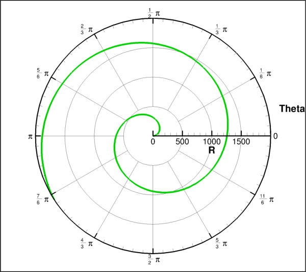
import numpy as np
import tecplot as tp
from tecplot.constant import *

frame = tp.active_frame()

npoints = 300
r = np.linspace(0, 2000, npoints)
theta = np.linspace(0, 10, npoints)

dataset = frame.create_dataset('Data', ['R', 'Theta'])
zone = dataset.add_ordered_zone('Zone', (300,))
zone.values('R')[:] = r
zone.values('Theta')[:] = theta

plot = frame.plot(PlotType.PolarLine)
plot.activate()
plot.axes.r_axis.max = r.max()
plot.axes.theta_axis.mode = ThetaMode.Radians
plot.delete_linemaps()
lmap = plot.add_linemap('Linemap', zone, dataset.variable('R'),
                            dataset.variable('Theta'))
lmap.line.line_thickness = 0.8
lmap.line.color = Color.Green

plot.view.fit()

tp.export.save_png('plot_polar.png', 600, supersample=3)

Attributes

`active_linemap_indices`	`set` of all active linemaps by index.
`active_linemaps`	Active linemaps in this plot.
`axes`	Axes style control for this plot.
`base_font`	Default typeface style control.
`data_labels`	Node and cell labels.
`legend`	Line plot legend style and placement control.
`linking_between_frames`	Style linking between frames.
`num_linemaps`	Number of linemaps held by this plot.
`show_lines`	Enable lines for this plot.
`show_symbols`	Enable symbols at line vertices for this plot.
`value_blanking`	Mask off points by value.
`view`	View control of the plot relative to the frame.

Methods

`activate`()	Make this the active plot type on the parent frame.
`activated`()	Context to ensure this plot is active.
`add_linemap`([name, zone, r, theta, show])	Add a linemap using the specified zone and variables.
`delete_linemaps`(*linemaps)	Clear all linemaps within this plot.
`linemap`(pattern)	Returns a specific linemap within this plot.
`linemaps`(*keys)	`PolarLinemapCollection` by index or name.

PolarLinePlot.activate()[source]¶

Make this the active plot type on the parent frame.

Example usage:

>>> from tecplot.constant import PlotType
>>> plot = frame.plot(PlotType.PolarLine)
>>> plot.activate()

PolarLinePlot.activated()¶

Context to ensure this plot is active.

Example usage:

>>> from tecplot.constant import PlotType
>>> frame = tecplot.active_frame()
>>> frame.plot_type = PlotType.XYLine  # set active plot type
>>> plot = frame.plot(PlotType.Cartesian3D)  # get inactive plot
>>> print(frame.plot_type)
PlotType.XYLine
>>> with plot.activated():
...     print(frame.plot_type)  # 3D plot temporarily active
PlotType.Cartesian3D
>>> print(frame.plot_type)  # original plot type restored
PlotType.XYLine

PolarLinePlot.active_linemap_indices¶

set of all active linemaps by index.

Numbers are zero-based indices to the linemaps:

>>> active_indices = plot.active_linemap_indices
>>> active_lmaps = [plot.linemap(i) for i in active_indices]

Type:: set of integers

PolarLinePlot.active_linemaps¶

Active linemaps in this plot.

Example usage:

>>> plot.active_linemaps.show_symbols = True

Type:: PolarLinemapCollection

PolarLinePlot.add_linemap(name=None, zone=None, r=None, theta=None, show=True)[source]¶

Add a linemap using the specified zone and variables.

Parameters:

name (str) – Name of the linemap which can be used for retrieving with PolarLinePlot.linemap. If None, then the linemap will not have a name. Default: None.
zone (Zone) – The data to be used when drawing this linemap. If None, then Tecplot Engine will select a Zone. Default: None.
r (Variable) – The r variable which must be from the same Dataset as theta and zone. If None, then Tecplot Engine will select a variable. Default: None.
theta (Variable) – The theta variable which must be from the same Dataset as r and zone. If None, then Tecplot Engine will select a variable. Default: None.
show (bool, optional) – Enable this linemap as soon as it’s added. (default: True)

Returns:

PolarLinemap

Example usage:

>>> lmap = plot.add_linemap('Line 1', dataset.zone('Zone'),
...                         dataset.variable('R'),
...                         dataset.variable('Theta'))
>>> lmap.line.line_thickness = 0.8

PolarLinePlot.axes¶

Axes style control for this plot.

Example usage:

>>> from tecplot.constant import PlotType, ThetaMode
>>> frame.plot_type = PlotType.PolarLine
>>> axes = frame.plot().axes
>>> axes.theta_mode = ThetaMode.Radians

Type:: PolarLineAxes

PolarLinePlot.base_font¶

Default typeface style control.

Example usage:

>>> plot.base_font.typeface = 'Times'

Type:: BaseFont

PolarLinePlot.data_labels¶

Node and cell labels.

This object controls displaying labels for every node and/or cell in the dataset. Example usage:

>>> plot.data_labels.show_node_labels = True
>>> plot.data_labels.step_index = 10

Type:: LinePlotDataLabels

PolarLinePlot.delete_linemaps(*linemaps)¶

Clear all linemaps within this plot.

Parameters:: *linemaps (Linemaps, int or str) – One or more of the following: Linemaps objects, linemap indices (zero-based) or linemap names. If none are given, all linemaps will be deleted.

Example usage:

>>> plot.delete_linemaps()
>>> print(plot.num_linemaps)
0

PolarLinePlot.legend¶

Line plot legend style and placement control.

Example usage:

>>> plot.legend.show = True

Type:: LineLegend

PolarLinePlot.linemap(pattern)[source]¶

Returns a specific linemap within this plot.

Parameters:: pattern (int, str or re.Pattern) – Zero-based index, case-insensitive glob-style pattern string or a compiled regex pattern instance used to match the linemaps by name. A negative index is interpreted as counting from the end of the available linemaps.
Returns:: PolarLinemap corresponding to pattern or None if pattern was passed in as a str or regex pattern instance and no matching linemap was found.

Note

Plots can contain linemaps with identical names and only the first match found is returned. This is not guaranteed to be deterministic and care should be taken to have only linemaps with unique names when this feature is used.

Example usage:

>>> plot.linemap(0).error_bar.show = True

PolarLinePlot.linemaps(*keys)[source]¶

PolarLinemapCollection by index or name.

Parameters:: keys (int, str or re.Pattern) – Zero-based index, case-insensitive glob-style pattern string or a compiled regex pattern instance used to match the linemaps by name. A negative index is interpreted as counting from the end of the available linemaps.

Example usage, adjusting the line thickness for all lines in the plot:

>>> plot.linemaps().line.line_thickness = 1.4

PolarLinePlot.linking_between_frames¶

Style linking between frames.

Example usage:

>>> plot.linking_between_frames.group = 1
>>> plot.linking_between_frames.link_solution_time = True

Type:: PolarPlotLinkingBetweenFrames

PolarLinePlot.num_linemaps¶

Number of linemaps held by this plot.

Example usage:

>>> print(plot.num_linemaps)
3

Type:: int

PolarLinePlot.show_lines¶

Enable lines for this plot.

Example usage:

>>> plot.show_lines = True

Type:: bool

PolarLinePlot.show_symbols¶

Enable symbols at line vertices for this plot.

Example usage:

>>> plot.show_symbols = True

Type:: bool

PolarLinePlot.value_blanking¶

Mask off points by value.

Example usage:

>>> plot.value_blanking.constraint(0).comparison_value = 3.14
>>> plot.value_blanking.constraint(0).active = True

Type:: ValueBlanking

PolarLinePlot.view¶

View control of the plot relative to the frame.

Example usage:

>>> plot.view.fit()

Type:: PolarView

XYLinePlot ¶

class tecplot.plot.XYLinePlot(frame)[source]¶

Cartesian plot with line data and associated style through linemaps.

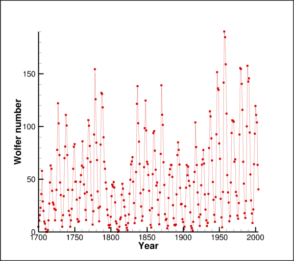
from os import path
import tecplot as tp
from tecplot.constant import PlotType, FillMode

examples_dir = tp.session.tecplot_examples_directory()
infile = path.join(examples_dir, 'SimpleData', 'SunSpots.plt')
dataset = tp.data.load_tecplot(infile)

frame = tp.active_frame()
plot = frame.plot(PlotType.XYLine)
plot.activate()
plot.show_symbols = True
plot.linemap(0).symbols.fill_mode = FillMode.UseLineColor
plot.linemap(0).symbols.size = 1

tp.export.save_png('plot_xyline.png', 600, supersample=3)

Attributes

`active_linemap_indices`	`set` of all active linemaps by index.
`active_linemaps`	Active linemaps in this plot.
`axes`	Axes style control for this plot.
`base_font`	Default typeface style control.
`data_labels`	Node and cell labels.
`legend`	Line plot legend style and placement control.
`linking_between_frames`	Style linking between frames.
`num_linemaps`	Number of linemaps held by this plot.
`show_bars`	Enable bar chart drawing mode for this plot.
`show_error_bars`	Enable error bars for this plot.
`show_lines`	Enable lines for this plot.
`show_symbols`	Enable symbols at line vertices for this plot.
`value_blanking`	Mask off points by value.
`view`	View control of the plot relative to the frame.

Methods

`activate`()	Make this the active plot type on the parent frame.
`activated`()	Context to ensure this plot is active.
`add_linemap`([name, zone, x, y, show])	Add a linemap using the specified zone and variables.
`delete_linemaps`(*linemaps)	Clear all linemaps within this plot.
`linemap`(pattern)	Returns a specific linemap within this plot.
`linemaps`(*keys)	`XYLinemapCollection` by index or name.

XYLinePlot.activate()[source]¶

Make this the active plot type on the parent frame.

Example usage:

>>> from tecplot.constant import PlotType
>>> plot = frame.plot(PlotType.XYLine)
>>> plot.activate()

XYLinePlot.activated()¶

Context to ensure this plot is active.

Example usage:

>>> from tecplot.constant import PlotType
>>> frame = tecplot.active_frame()
>>> frame.plot_type = PlotType.XYLine  # set active plot type
>>> plot = frame.plot(PlotType.Cartesian3D)  # get inactive plot
>>> print(frame.plot_type)
PlotType.XYLine
>>> with plot.activated():
...     print(frame.plot_type)  # 3D plot temporarily active
PlotType.Cartesian3D
>>> print(frame.plot_type)  # original plot type restored
PlotType.XYLine

XYLinePlot.active_linemap_indices¶

set of all active linemaps by index.

Numbers are zero-based indices to the linemaps:

>>> active_indices = plot.active_linemap_indices
>>> active_lmaps = [plot.linemap(i) for i in active_indices]

Type:: set of integers

XYLinePlot.active_linemaps¶

Active linemaps in this plot.

Example usage:

>>> plot.active_linemaps.show_symbols = True

Type:: XYLinemapCollection

XYLinePlot.add_linemap(name=None, zone=None, x=None, y=None, show=True)[source]¶

Add a linemap using the specified zone and variables.

Parameters:

name (str) – Name of the linemap which can be used for retrieving with XYLinePlot.linemap. If None, then the linemap will not have a name. Default: None.
zone (Zone) – The data to be used when drawing this linemap. If None, then Tecplot Engine will select a zone. Default: None.
x (Variable) – The x variable which must be from the same Dataset as y and zone. If None, then Tecplot Engine will select an x variable. Default: None.
y (Variable) – The y variable which must be from the same Dataset as x and zone. If None, then Tecplot Engine will select a y variable. Default: None.
show (bool, optional) – Enable this linemap as soon as it’s added. (default: True). If None, then Tecplot Engine will determine if the linemap should be enabled.

Returns:

XYLinemap

Example usage:

>>> lmap = plot.add_linemap('Line 1', dataset.zone('Zone'),
...                         dataset.variable('X'),
...                         dataset.variable('Y'))
>>> lmap.line.line_thickness = 0.8

XYLinePlot.axes¶

Axes style control for this plot.

Example usage:

>>> from tecplot.constant import PlotType, AxisMode
>>> frame.plot_type = PlotType.XYLine
>>> axes = frame.plot().axes
>>> axes.axis_mode = AxisMode.XYDependent
>>> axes.xy_ratio = 2

Type:: XYLineAxes

XYLinePlot.base_font¶

Default typeface style control.

Example usage:

>>> plot.base_font.typeface = 'Times'

Type:: BaseFont

XYLinePlot.data_labels¶

Node and cell labels.

This object controls displaying labels for every node and/or cell in the dataset. Example usage:

>>> plot.data_labels.show_node_labels = True
>>> plot.data_labels.step_index = 10

Type:: LinePlotDataLabels

XYLinePlot.delete_linemaps(*linemaps)¶

Clear all linemaps within this plot.

Parameters:: *linemaps (Linemaps, int or str) – One or more of the following: Linemaps objects, linemap indices (zero-based) or linemap names. If none are given, all linemaps will be deleted.

Example usage:

>>> plot.delete_linemaps()
>>> print(plot.num_linemaps)
0

XYLinePlot.legend¶

Line plot legend style and placement control.

Example usage:

>>> plot.legend.show = True

Type:: LineLegend

XYLinePlot.linemap(pattern)[source]¶

Returns a specific linemap within this plot.

Parameters:: pattern (int, str or re.Pattern) – Zero-based index, case-insensitive glob-style pattern string or a compiled regex pattern instance used to match the linemaps by name. A negative index is interpreted as counting from the end of the available linemaps.
Returns:: XYLinemap corresponding to pattern or None if pattern was passed in as a str or regex pattern instance and no matching linemap was found.

Note

Plots can contain linemaps with identical names and only the first match found is returned. This is not guaranteed to be deterministic and care should be taken to have only linemaps with unique names when this feature is used.

Example usage:

>>> plot.linemap(0).error_bar.show = True

XYLinePlot.linemaps(*keys)[source]¶

XYLinemapCollection by index or name.

Parameters:: keys (int, str or re.Pattern) – Zero-based index, case-insensitive glob-style pattern string or a compiled regex pattern instance used to match the linemaps by name. A negative index is interpreted as counting from the end of the available linemaps.

Example usage, adjusting the line thickness for all lines in the plot:

>>> plot.linemaps().line.line_thickness = 1.4

XYLinePlot.linking_between_frames¶

Style linking between frames.

Example usage:

>>> plot.linking_between_frames.group = 1
>>> plot.linking_between_frames.link_solution_time = True

Type:: XYLinePlotLinkingBetweenFrames

XYLinePlot.num_linemaps¶

Number of linemaps held by this plot.

Example usage:

>>> print(plot.num_linemaps)
3

Type:: int

XYLinePlot.show_bars¶

Enable bar chart drawing mode for this plot.

Example usage:

>>> plot.show_bars = True

Type:: bool

XYLinePlot.show_error_bars¶

Enable error bars for this plot.

The variable to be used for error bars must be set first on at least one linemap within this plot:

>>> plot.linemap(0).error_bars.variable = dataset.variable('E')
>>> plot.show_error_bars = True

Type:: bool

XYLinePlot.show_lines¶

Enable lines for this plot.

Example usage:

>>> plot.show_lines = True

Type:: bool

XYLinePlot.show_symbols¶

Enable symbols at line vertices for this plot.

Example usage:

>>> plot.show_symbols = True

Type:: bool

XYLinePlot.value_blanking¶

Mask off points by value.

Example usage:

>>> plot.value_blanking.constraint(0).comparison_value = 3.14
>>> plot.value_blanking.constraint(0).active = True

Type:: ValueBlanking

XYLinePlot.view¶

View control of the plot relative to the frame.

Example usage:

>>> plot.view.fit()

Type:: XYLineView

SketchPlot ¶

class tecplot.plot.SketchPlot(frame, *svargs)[source]¶

A plot space with no data attached.

import tecplot as tp
from tecplot.constant import PlotType

frame = tp.active_frame()
plot = frame.plot(PlotType.Sketch)

frame.add_text('Hello, World!', (36, 50), size=34)
plot.axes.x_axis.show = True
plot.axes.y_axis.show = True

tp.export.save_png('plot_sketch.png', 600, supersample=3)

Attributes

`axes`	Axes (x and y) for the sketch plot.
`linking_between_frames`	Style linking between frames.

Methods

`activate`()	Make this the active plot type on the parent frame.
`activated`()	Context to ensure this plot is active.

SketchPlot.activate()[source]¶

Make this the active plot type on the parent frame.

Example usage:

>>> from tecplot.constant import PlotType
>>> plot = frame.plot(PlotType.Sketch)
>>> plot.activate()

SketchPlot.activated()¶

Context to ensure this plot is active.

Example usage:

>>> from tecplot.constant import PlotType
>>> frame = tecplot.active_frame()
>>> frame.plot_type = PlotType.XYLine  # set active plot type
>>> plot = frame.plot(PlotType.Cartesian3D)  # get inactive plot
>>> print(frame.plot_type)
PlotType.XYLine
>>> with plot.activated():
...     print(frame.plot_type)  # 3D plot temporarily active
PlotType.Cartesian3D
>>> print(frame.plot_type)  # original plot type restored
PlotType.XYLine

SketchPlot.axes¶

Axes (x and y) for the sketch plot.

Example usage:

>>> from tecplot.constant import PlotType
>>> frame.plot_type = PlotType.Sketch
>>> frame.plot().axes.x_axis.show = True

Type:: SketchAxes

SketchPlot.linking_between_frames¶

Style linking between frames.

Example usage:

>>> plot.linking_between_frames.group = 1
>>> plot.linking_between_frames.link_solution_time = True

Type:: SketchPlotLinkingBetweenFrames

Fieldmaps ¶

Cartesian2DFieldmap ¶

class tecplot.plot.Cartesian2DFieldmap(plot, index)[source]¶

Style control for a single 2D fieldmap.

See also

Cartesian2DFieldmapCollection

Attributes

`contour`	Style including flooding, lines and line coloring.
`edge`	Style control for boundary lines.
`effects`	Style control for clipping and blanking effects.
`fieldmap_indices`	Read-only, sorted `list` of zero-based fieldmap indices.
`group`	Zero-based group number for this Fieldmaps.
`mesh`	Style lines connecting neighboring data points.
`points`	Control which points to draw.
`scatter`	Style for scatter plots.
`shade`	Style control for surface shading.
`show`	Display this fieldmap on the plot.
`surfaces`	Control which surfaces to draw.
`vector`	Style for vector field plots using arrows.
`zones`	List of zones used by this fieldmap.

Cartesian2DFieldmap.contour¶

Style including flooding, lines and line coloring.

Type:: FieldmapContour

Cartesian2DFieldmap.edge¶

Style control for boundary lines.

Type:: FieldmapEdge

Cartesian2DFieldmap.effects¶

Style control for clipping and blanking effects.

Type:: FieldmapEffects

Cartesian2DFieldmap.fieldmap_indices¶

Read-only, sorted list of zero-based fieldmap indices.

Type:: list

Cartesian2DFieldmap.group¶

Zero-based group number for this Fieldmaps.

This is a piece of auxiliary data and can be useful for identifying a subset of fieldmaps. For example, to loop over all fieldmaps that have group set to 4:

>>> plot.fieldmaps(0, 3).group = 4
>>> for fmap in filter(lambda f: f.group == 4, plot.fieldmaps()):
...     print(fmap.index)
0
3

Type:: int

Cartesian2DFieldmap.mesh¶

Style lines connecting neighboring data points.

Type:: FieldmapMesh

Cartesian2DFieldmap.points¶

Control which points to draw.

Type:: FieldmapPoints

Cartesian2DFieldmap.scatter¶

Style for scatter plots.

Type:: FieldmapScatter

Cartesian2DFieldmap.shade¶

Style control for surface shading.

Type:: FieldmapShade

Cartesian2DFieldmap.show¶

Display this fieldmap on the plot.

Example usage:

>>> plot.fieldmap(0).show = True

For optimized style control of several fieldmaps, it is recommended to use Cartesian2DFieldmapCollection or Cartesian3DFieldmapCollection objects.

Type:: bool

Cartesian2DFieldmap.surfaces¶

Control which surfaces to draw.

Type:: FieldmapSurfaces

Cartesian2DFieldmap.vector¶

Style for vector field plots using arrows.

Type:: FieldmapVector

Cartesian2DFieldmap.zones¶

List of zones used by this fieldmap.

Example usage:

>>> for zone in fieldmap.zones:
...     print(zone.name)
Zone 1
Zone 2

Cartesian2DFieldmapCollection ¶

class tecplot.plot.Cartesian2DFieldmapCollection(plot, *indices)[source]¶

Style control for one or more 2D fieldmaps.

This class behaves like Cartesian2DFieldmap except that setting any underlying style will do so for all of the represented fieldmaps. The style properties are then always returned as a tuple of properties, one for each fieldmap, ordered by index number. This means there is an asymmetry between setting and getting any property under this object, illustrated by the following example:

>>> fmaps = plot.fieldmaps(0, 1, 2)
>>> fmaps.show = True
>>> print(fmaps.show)
(True, True, True)

This is the preferred way to control the style of many fieldmaps as it is much faster to execute. All examples that set style on a single fieldmap like the following:

>>> plot.fieldmap(0).contour.show = True

may be converted to setting the same style on all fieldmaps like so:

>>> plot.fieldmaps().contour.show = True

See also

Cartesian2DFieldmap

New in version 1.1: Fieldmap collection objects.

Attributes

`contour`	Style including flooding, lines and line coloring.
`edge`	Style control for boundary lines.
`effects`	Style control for clipping and blanking effects.
`fieldmap_indices`	Read-only, sorted `list` of zero-based fieldmap indices.
`group`	Zero-based group number for this Fieldmaps.
`mesh`	Style lines connecting neighboring data points.
`points`	Control which points to draw.
`scatter`	Style for scatter plots.
`shade`	Style control for surface shading.
`show`	Display the fielmaps in this collection on the plot.
`surfaces`	Control which surfaces to draw.
`vector`	Style for vector field plots using arrows.

Cartesian2DFieldmapCollection.contour¶

Style including flooding, lines and line coloring.

Type:: FieldmapContour

Cartesian2DFieldmapCollection.edge¶

Style control for boundary lines.

Type:: FieldmapEdge

Cartesian2DFieldmapCollection.effects¶

Style control for clipping and blanking effects.

Type:: FieldmapEffects

Cartesian2DFieldmapCollection.fieldmap_indices¶

Read-only, sorted list of zero-based fieldmap indices.

Type:: list

Cartesian2DFieldmapCollection.group¶

Zero-based group number for this Fieldmaps.

This is a piece of auxiliary data and can be useful for identifying a subset of fieldmaps. For example, to loop over all fieldmaps that have group set to 4:

>>> plot.fieldmaps(0, 3).group = 4
>>> for fmap in filter(lambda f: f.group == 4, plot.fieldmaps()):
...     print(fmap.index)
0
3

Type:: int

Cartesian2DFieldmapCollection.mesh¶

Style lines connecting neighboring data points.

Type:: FieldmapMesh

Cartesian2DFieldmapCollection.points¶

Control which points to draw.

Type:: FieldmapPoints

Cartesian2DFieldmapCollection.scatter¶

Style for scatter plots.

Type:: FieldmapScatter

Cartesian2DFieldmapCollection.shade¶

Style control for surface shading.

Type:: FieldmapShade

Cartesian2DFieldmapCollection.show¶

Display the fielmaps in this collection on the plot.

Example turning on all fieldmaps on the plot:

>>> plot.fieldmaps().show = True

Type:: bool

Cartesian2DFieldmapCollection.surfaces¶

Control which surfaces to draw.

Type:: FieldmapSurfaces

Cartesian2DFieldmapCollection.vector¶

Style for vector field plots using arrows.

Type:: FieldmapVector

Cartesian3DFieldmap ¶

class tecplot.plot.Cartesian3DFieldmap(plot, index)[source]¶

Style control for a single 3D fieldmap.

See also

Cartesian3DFieldmapCollection

Attributes

`contour`	Style including flooding, lines and line coloring.
`edge`	Style control for boundary lines.
`effects`	Style control for blanking and lighting effects.
`fieldmap_indices`	Read-only, sorted `list` of zero-based fieldmap indices.
`group`	Zero-based group number for this Fieldmaps.
`mesh`	Style lines connecting neighboring data points.
`points`	Control which points to draw.
`scatter`	Style for scatter plots.
`shade`	Style control for surface shading.
`show`	Display this fieldmap on the plot.
`show_isosurfaces`	Enable drawing of Iso-surfaces.
`show_slices`	Enable drawing of slice surfaces.
`show_streamtraces`	Enable drawing of streamtraces.
`surfaces`	Control which surfaces to draw.
`vector`	Style for vector field plots using arrows.
`zones`	List of zones used by this fieldmap.

Cartesian3DFieldmap.contour¶

Style including flooding, lines and line coloring.

Type:: FieldmapContour

Cartesian3DFieldmap.edge¶

Style control for boundary lines.

Type:: FieldmapEdge

Cartesian3DFieldmap.effects¶

Style control for blanking and lighting effects.

Type:: FieldmapEffects3D

Cartesian3DFieldmap.fieldmap_indices¶

Read-only, sorted list of zero-based fieldmap indices.

Type:: list

Cartesian3DFieldmap.group¶

Zero-based group number for this Fieldmaps.

This is a piece of auxiliary data and can be useful for identifying a subset of fieldmaps. For example, to loop over all fieldmaps that have group set to 4:

>>> plot.fieldmaps(0, 3).group = 4
>>> for fmap in filter(lambda f: f.group == 4, plot.fieldmaps()):
...     print(fmap.index)
0
3

Type:: int

Cartesian3DFieldmap.mesh¶

Style lines connecting neighboring data points.

Type:: FieldmapMesh

Cartesian3DFieldmap.points¶

Control which points to draw.

Type:: FieldmapPoints

Cartesian3DFieldmap.scatter¶

Style for scatter plots.

Type:: FieldmapScatter

Cartesian3DFieldmap.shade¶

Style control for surface shading.

Type:: FieldmapShade3D

Cartesian3DFieldmap.show¶

Display this fieldmap on the plot.

Example usage:

>>> plot.fieldmap(0).show = True

For optimized style control of several fieldmaps, it is recommended to use Cartesian2DFieldmapCollection or Cartesian3DFieldmapCollection objects.

Type:: bool

Cartesian3DFieldmap.show_isosurfaces¶

Enable drawing of Iso-surfaces.

Type:: bool

Cartesian3DFieldmap.show_slices¶

Enable drawing of slice surfaces.

Type:: bool

Cartesian3DFieldmap.show_streamtraces¶

Enable drawing of streamtraces.

Type:: bool

Cartesian3DFieldmap.surfaces¶

Control which surfaces to draw.

Type:: FieldmapSurfaces

Cartesian3DFieldmap.vector¶

Style for vector field plots using arrows.

Type:: FieldmapVector

Cartesian3DFieldmap.zones¶

List of zones used by this fieldmap.

Example usage:

>>> for zone in fieldmap.zones:
...     print(zone.name)
Zone 1
Zone 2

Cartesian3DFieldmapCollection ¶

class tecplot.plot.Cartesian3DFieldmapCollection(plot, *indices)[source]¶

Style control for one or more 3D fieldmaps.

This class behaves like Cartesian3DFieldmap except that setting any underlying style will do so for all of the represented fieldmaps. The style properties are then always returned as a tuple of properties, one for each fieldmap, ordered by index number. This means there is an asymmetry between setting and getting any property under this object, illustrated by the following example:

>>> fmaps = plot.fieldmaps(0, 1, 2)
>>> fmaps.show = True
>>> print(fmaps.show)
(True, True, True)

This is the preferred way to control the style of many fieldmaps as it is much faster to execute. All examples that set style on a single fieldmap like the following:

>>> plot.fieldmap(0).contour.show = True

may be converted to setting the same style on all fieldmaps like so:

>>> plot.fieldmaps().contour.show = True

See also

Cartesian3DFieldmap

New in version 1.1: Fieldmap collection objects.

The following example illustrates manipulating the style for a selection of fieldmaps associated with specific zones:

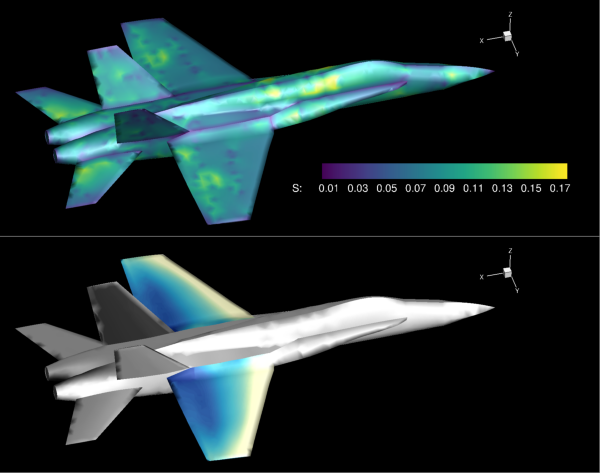
import os
import numpy
import tecplot

examples_dir = tecplot.session.tecplot_examples_directory()
infile = os.path.join(examples_dir, 'SimpleData', 'F18.lay')
tecplot.load_layout(infile)
frame = tecplot.active_frame()
plot = frame.plot()
dataset = frame.dataset

plot.contour(0).colormap_name = 'GrayScale'
plot.contour(0).legend.show = False

wings = [dataset.zone(name) for name in ['left wing', 'right wing']]
fmaps = frame.plot().fieldmaps(wings)
fmaps.contour.flood_contour_group = plot.contour(1)

plot.contour(1).colormap_name = 'Sequential - Yellow/Green/Blue'
plot.contour(1).levels.reset_levels(numpy.linspace(-0.07, 0.07, 50))

tecplot.export.save_png('F18_wings.png', 600, supersample=3)

Attributes

`contour`	Style including flooding, lines and line coloring.
`edge`	Style control for boundary lines.
`effects`	Style control for blanking and lighting effects.
`fieldmap_indices`	Read-only, sorted `list` of zero-based fieldmap indices.
`group`	Zero-based group number for this Fieldmaps.
`mesh`	Style lines connecting neighboring data points.
`points`	Control which points to draw.
`scatter`	Style for scatter plots.
`shade`	Style control for surface shading.
`show`	Display the fielmaps in this collection on the plot.
`show_isosurfaces`	Enable drawing of Iso-surfaces.
`show_slices`	Enable drawing of slice surfaces.
`show_streamtraces`	Enable drawing of streamtraces.
`surfaces`	Control which surfaces to draw.
`vector`	Style for vector field plots using arrows.

Cartesian3DFieldmapCollection.contour¶

Style including flooding, lines and line coloring.

Type:: FieldmapContour

Cartesian3DFieldmapCollection.edge¶

Style control for boundary lines.

Type:: FieldmapEdge

Cartesian3DFieldmapCollection.effects¶

Style control for blanking and lighting effects.

Type:: FieldmapEffects3D

Cartesian3DFieldmapCollection.fieldmap_indices¶

Read-only, sorted list of zero-based fieldmap indices.

Type:: list

Cartesian3DFieldmapCollection.group¶

Zero-based group number for this Fieldmaps.

This is a piece of auxiliary data and can be useful for identifying a subset of fieldmaps. For example, to loop over all fieldmaps that have group set to 4:

>>> plot.fieldmaps(0, 3).group = 4
>>> for fmap in filter(lambda f: f.group == 4, plot.fieldmaps()):
...     print(fmap.index)
0
3

Type:: int

Cartesian3DFieldmapCollection.mesh¶

Style lines connecting neighboring data points.

Type:: FieldmapMesh

Cartesian3DFieldmapCollection.points¶

Control which points to draw.

Type:: FieldmapPoints

Cartesian3DFieldmapCollection.scatter¶

Style for scatter plots.

Type:: FieldmapScatter

Cartesian3DFieldmapCollection.shade¶

Style control for surface shading.

Type:: FieldmapShade3D

Cartesian3DFieldmapCollection.show¶

Display the fielmaps in this collection on the plot.

Example turning on all fieldmaps on the plot:

>>> plot.fieldmaps().show = True

Type:: bool

Cartesian3DFieldmapCollection.show_isosurfaces¶

Enable drawing of Iso-surfaces.

Type:: bool

Cartesian3DFieldmapCollection.show_slices¶

Enable drawing of slice surfaces.

Type:: bool

Cartesian3DFieldmapCollection.show_streamtraces¶

Enable drawing of streamtraces.

Type:: bool

Cartesian3DFieldmapCollection.surfaces¶

Control which surfaces to draw.

Type:: FieldmapSurfaces

Cartesian3DFieldmapCollection.vector¶

Style for vector field plots using arrows.

Type:: FieldmapVector

FieldmapContour ¶

class tecplot.plot.FieldmapContour(fieldmap)[source]¶

Style control for flooding and contour lines.

This object controls which contour groups are associated with flooding, line placement and line coloring. Three different contour groups may be used though there are eight total groups that can be configured in a single plot. In this example, we flood by the first contour group (index: 0):

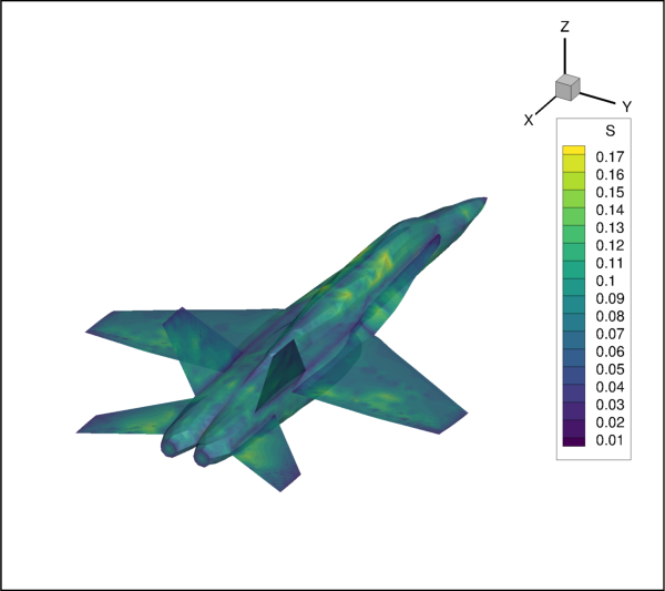
import numpy as np

import tecplot as tp
from tecplot.constant import *
from tecplot.data.operate import execute_equation

# Get the active frame, setup a grid (30x30x30)
# where each dimension ranges from 0 to 30.
# Add variables P,Q,R to the dataset and give
# values to the data.
frame = tp.active_frame()
dataset = frame.dataset
for v in ['X','Y','Z','P','Q','R']:
    dataset.add_variable(v)
zone = dataset.add_ordered_zone('Zone', (30,30,30))
xx = np.linspace(0,30,30)
for v,arr in zip(['X','Y','Z'],np.meshgrid(xx,xx,xx)):
    zone.values(v)[:] = arr.ravel()
execute_equation('{P} = -10 * {X}    +      {Y}**2 + {Z}**2')
execute_equation('{Q} =       {X}    - 10 * {Y}    - {Z}**2')
execute_equation('{R} =       {X}**2 +      {Y}**2 - {Z}   ')

# Enable 3D field plot and turn on contouring
# with boundary faces
frame.plot_type = PlotType.Cartesian3D
plot = frame.plot()
srf = plot.fieldmap(0).surfaces
srf.surfaces_to_plot = SurfacesToPlot.BoundaryFaces
plot.show_contour = True

# get the contour group associated with the
# newly created zone
contour = plot.fieldmap(dataset.zone('Zone')).contour

# assign flooding to the first contour group
contour.flood_contour_group = plot.contour(0)
contour.flood_contour_group.variable = dataset.variable('P')
contour.flood_contour_group.colormap_name = 'Sequential - Yellow/Green/Blue'
contour.flood_contour_group.legend.show = False

# save image to PNG file
tp.export.save_png('fieldmap_contour.png', 600, supersample=3)

Attributes

`contour_type`	`ContourType` to plot.
`flood_contour_group`	The `ContourGroup` to use for flooding.
`flood_contour_group_index`	Zero-based `Index` of the `ContourGroup` to use for flooding.
`line_color`	The `Color` or `ContourGroup` for lines.
`line_group`	`ContourGroup` to use for line placement and style.
`line_group_index`	Zero-based `Index` of the `ContourGroup` for contour lines.
`line_pattern`	`LinePattern` type to use for contour lines.
`line_thickness`	Thickness (`float`) of the drawn lines.
`pattern_length`	Length (`float`) of the pattern segment for non-solid lines.
`show`	Enable drawing the contours.
`use_lighting_effect`	Enable lighting effect on this contour.

FieldmapContour.contour_type¶

ContourType to plot.

Possible values are:

ContourType.Flood (default)
Filled color between the contour levels.

ContourType.Lines
Lines only.

ContourType.Overlay
Lines overlayed on flood.

ContourType.AverageCell
Filled color by the average value within cells.

ContourType.PrimaryValue
Filled color by the value at the primary corner of the cells.

In this example, we enable both flooding and contour lines:

>>> from tecplot.constant import ContourType
>>> contour = plot.fieldmap(0).contour
>>> contour.contour_type = ContourType.Overlay

Type:: ContourType

FieldmapContour.flood_contour_group¶

The ContourGroup to use for flooding.

This property sets and gets the ContourGroup used for flooding. Changing style on this ContourGroup will affect all other fieldmaps on the same Frame that use it. Example usage:

>>> cmap_name = 'Sequential - Yellow/Green/Blue'
>>> contour = plot.fieldmap(0).contour
>>> contour.flood_contour_group = plot.contour(1)
>>> contour.flood_contour_group.variable = dataset.variable('P')
>>> contour.flood_contour_group.colormap_name = cmap_name

Setting this to the RGBColoring instance floods this fieldmap contour by the plot’s RGB coloring settings. This requires that variables are assigned to the red, green and blue color channels:

>>> plot.rgb_coloring.red_variable = dataset.variable('x')
>>> plot.rgb_coloring.green_variable = dataset.variable('y')
>>> plot.rgb_coloring.blue_variable = dataset.variable('z')
>>> contour = plot.fieldmap(0).contour
>>> contour.flood_contour_group = plot.rgb_coloring

See RGBColoring for more details.

Type:: ContourGroup or RGBColoring

FieldmapContour.flood_contour_group_index¶

Zero-based Index of the ContourGroup to use for flooding.

This property sets and gets, by Index, the ContourGroup used for flooding. Changing style on this ContourGroup will affect all other fieldmaps on the same Frame that use it. Example usage:

>>> contour = plot.fieldmap(0).contour
>>> contour.flood_contour_group_index = 1
>>> contour.flood_contour_group.variable = dataset.variable('P')

Note

To set the flood contour to RGB (multivariate) coloring, you must set the FieldmapContour.flood_contour_group property to plot.rgb_coloring. See FieldmapContour.flood_contour_group for more details.

Type:: int

FieldmapContour.line_color¶

The Color or ContourGroup for lines.

FieldmapContour lines can be a solid color or be colored by a ContourGroup as obtained through the plot.contour property. Note that changing style on this ContourGroup will affect all other fieldmaps on the same Frame that use it. Example usage:

>>> from tecplot.constant import Color
>>> contour = plot.fieldmap(1).contour
>>> contour.line_color = Color.Blue

Example of setting the color from a ContourGroup:

>>> contour = plot.fieldmap(0).contour
>>> contour.line_color = plot.contour(1)
>>> contour.line_color.variable = dataset.variable('P')

Setting this to the RGBColoring instance colors the lines by the plot’s multivariate contour settings. This requires that variables are assigned to the red, green and blue color channels:

>>> plot.rgb_coloring.red_variable = dataset.variable('x')
>>> plot.rgb_coloring.green_variable = dataset.variable('y')
>>> plot.rgb_coloring.blue_variable = dataset.variable('z')
>>> plot.fieldmap(0).contour.line_color = plot.rgb_coloring

See RGBColoring for more details.

Type:: Color or ContourGroup

FieldmapContour.line_group¶

ContourGroup to use for line placement and style.

This property sets and gets the ContourGroup used for line placement and though all properties of the ContourGroup can be manipulated through this object, many of them such as color will not effect the lines unless the FieldmapContour.line_color is set to the same ContourGroup. Note that changing style on this ContourGroup will affect all other fieldmaps on the same Frame that use it. Example usage:

>>> contour = plot.fieldmap(0).contour
>>> contour.line_group = plot.contour(2)
>>> contour.line_group.variable = dataset.variable('Z')

Type:: ContourGroup

FieldmapContour.line_group_index¶

Zero-based Index of the ContourGroup for contour lines.

This property sets and gets, by Index, the ContourGroup used for line placement and though all properties of the ContourGroup can be manipulated through this object, many of them such as color will not affect the lines unless the FieldmapContour.line_color is set to the same ContourGroup. Note that changing style on this ContourGroup will affect all other fieldmaps on the same Frame that use it. Example usage:

>>> contour = plot.fieldmap(0).contour
>>> contour.line_group_index = 2
>>> contour.line_group.variable = dataset.variable('Z')

Type:: int

FieldmapContour.line_pattern¶

LinePattern type to use for contour lines.

Possible values: Solid, Dashed, DashDot, Dotted, LongDash, DashDotDot.

Example usage:

>>> from tecplot.constant import LinePattern
>>> contour = plot.fieldmap(0).contour
>>> contour.line_pattern = LinePattern.DashDotDot

Type:: LinePattern

FieldmapContour.line_thickness¶

Thickness (float) of the drawn lines.

This is the line thickness in percentage of the Frame’s height. Example usage:

>>> contour = plot.fieldmap(0).contour
>>> contour.line_thickness = 0.7

Type:: float

FieldmapContour.pattern_length¶

Length (float) of the pattern segment for non-solid lines.

This is the pattern length in percentage of the Frame’s height. Example usage:

>>> contour = plot.fieldmap(0).contour
>>> contour.pattern_length = 3.5

Type:: float

FieldmapContour.show¶

Enable drawing the contours.

Example usage:

>>> contour = plot.fieldmap(0).contour
>>> contour.show = True

Type:: bool

FieldmapContour.use_lighting_effect¶

Enable lighting effect on this contour.

Example usage:

>>> contour = plot.fieldmap(0).contour
>>> contour.use_lighting_effect = False

Type:: bool

FieldmapEdge ¶

class tecplot.plot.FieldmapEdge(fieldmap)[source]¶

Volume boundary lines.

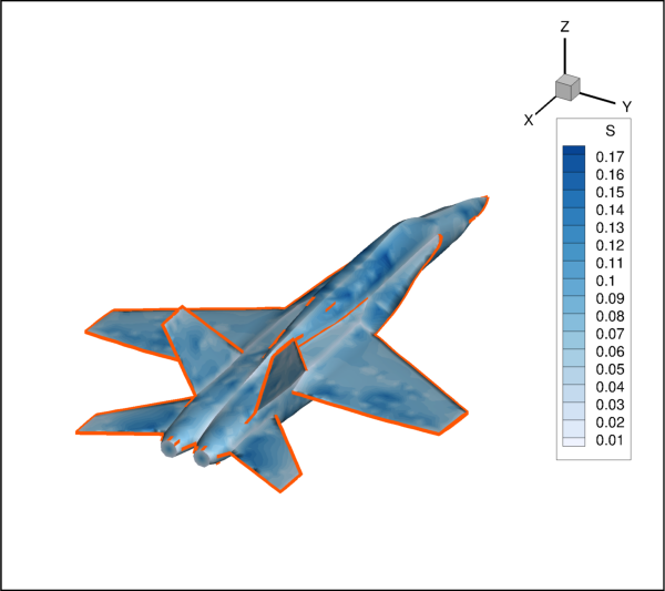
An edge plot layer displays the connections of the outer lines (IJ-ordered zones), finite element surface zones, or planes (IJK-ordered zones). The FieldmapEdge layer allows you to display the edges (creases and borders) of your data. Zone edges exist only for ordered zones or 2D finite element zones. Three-dimensional finite element zones do not have boundaries:

import os

import tecplot as tp
from tecplot.constant import Color, EdgeType, PlotType, SurfacesToPlot

examples_dir = tp.session.tecplot_examples_directory()
datafile = os.path.join(examples_dir, 'SimpleData', 'F18.plt')
dataset = tp.data.load_tecplot(datafile)
frame = dataset.frame

# Enable 3D field plot, turn on contouring and translucency
frame.plot_type = PlotType.Cartesian3D
plot = frame.plot()
plot.show_contour = True
plot.show_edge = True

contour = plot.contour(0)
contour.colormap_name = 'Sequential - Blue'
contour.variable = dataset.variable('S')

# adjust effects for every fieldmap in this dataset
fmaps = plot.fieldmaps()
fmaps.contour.flood_contour_group = contour
fmaps.surfaces.surfaces_to_plot = SurfacesToPlot.BoundaryFaces

edge = fmaps.edge
edge.edge_type = EdgeType.Creases
edge.color = Color.RedOrange
edge.line_thickness = 0.7

# ensure consistent output between interactive (connected) and batch
plot.contour(0).levels.reset_to_nice()

# save image to file
tp.export.save_png('fieldmap_edge.png', 600, supersample=3)

Attributes

`color`	Line `Color`.
`edge_type`	Where to draw edge lines.
`i_border`	Which border lines to draw in the `I`-dimension.
`j_border`	Which border lines to draw in the `J`-dimension.
`k_border`	Which border lines to draw in the `K`-dimension.
`line_thickness`	Thickness of the edge lines drawn.
`show`	Draw the mesh for this fieldmap.

FieldmapEdge.color¶

Line Color.

Type:: Color

FieldmapEdge.edge_type¶

Where to draw edge lines.

Possible values: Borders, Creases, BordersAndCreases.

Example usage:

>>> from tecplot.constant import EdgeType
>>> plot.show_edge = True
>>> plot.fieldmap(0).edge.edge_type = EdgeType.Creases

Type:: EdgeType

FieldmapEdge.i_border¶

Which border lines to draw in the I-dimension.

Possible values: None, Min, Max, Both.

Example usage:

>>> from tecplot.constant import BorderLocation
>>> plot.show_edge = True
>>> plot.fieldmap(0).edge.i_border = BorderLocation.Min

Type:: BorderLocation

FieldmapEdge.j_border¶

Which border lines to draw in the J-dimension.

Possible values: None, Min, Max, Both.

Example usage:

>>> from tecplot.constant import BorderLocation
>>> plot.show_edge = True
>>> plot.fieldmap(0).edge.j_border = BorderLocation.Both

Type:: BorderLocation

FieldmapEdge.k_border¶

Which border lines to draw in the K-dimension.

Possible values: None, Min, Max, Both.

Example usage:

>>> from tecplot.constant import BorderLocation
>>> plot.show_edge = True
>>> plot.fieldmap(0).edge.k_border = None

Type:: BorderLocation

FieldmapEdge.line_thickness¶

Thickness of the edge lines drawn.

This is the line thickness in percentage of Frame height. Example usage:

>>> plot.fieldmap(0).edge.line_thickness = 0.4

Type:: float

FieldmapEdge.show¶

Draw the mesh for this fieldmap.

Example usage:

>>> plot.show_edge = True
>>> plot.fieldmap(0).edge.show = True

Type:: bool

FieldmapEffects ¶

class tecplot.plot.FieldmapEffects(fieldmap)[source]¶

Clipping and blanking style control.

This object controls value blanking and clipping from plane slices for this fieldmap.

Attributes

`clip_planes`
`value_blanking`	Enable value blanking effect for this fieldmap.

FieldmapEffects.clip_planes¶

FieldmapEffects.value_blanking¶

Enable value blanking effect for this fieldmap.

Example usage:

>>> plot.fieldmap(0).effects.value_blanking = True

Type:: bool

FieldmapEffects3D ¶

class tecplot.plot.FieldmapEffects3D(fieldmap)[source]¶

Lighting and translucency style control.

import os

import tecplot as tp
from tecplot.constant import LightingEffect, PlotType, SurfacesToPlot

examples_dir = tp.session.tecplot_examples_directory()
datafile = os.path.join(examples_dir, 'SimpleData', 'F18.plt')
dataset = tp.data.load_tecplot(datafile)
frame = dataset.frame

# Enable 3D field plot, turn on contouring and translucency
frame.plot_type = PlotType.Cartesian3D
plot = frame.plot()
plot.show_contour = True
plot.use_translucency = True

plot.contour(0).variable = dataset.variable('S')

# adjust effects for every fieldmap in this dataset
fmaps = plot.fieldmaps()
fmaps.contour.flood_contour_group = plot.contour(0)
fmaps.surfaces.surfaces_to_plot = SurfacesToPlot.BoundaryFaces

eff = fmaps.effects
eff.lighting_effect = LightingEffect.Paneled
eff.surface_translucency = 30

# ensure consistent output between interactive (connected) and batch
plot.contour(0).levels.reset_to_nice()

# save image to file
tp.export.save_png('fieldmap_effects3d.png', 600, supersample=3)

Attributes

`clip_planes`	Slice groups to use for clipping.
`lighting_effect`	The type of lighting effect to render.
`surface_translucency`	`int` Translucency of all surfaces for this fieldmap in percent.
`use_translucency`	Enable translucency of all drawn surfaces for this fieldmap.
`value_blanking`	Enable value blanking effect for this fieldmap.

FieldmapEffects3D.clip_planes¶

Slice groups to use for clipping.

Only slice groups 0 to 5 are available for clipping. Example usage:

>>> plot.fieldmap(0).effects.clip_planes = [0, 1, 2]

See also

SliceGroup.clip

Type:: list of integers [0-5]

FieldmapEffects3D.lighting_effect¶

The type of lighting effect to render.

Possible values:

Paneled: Within each cell, the color assigned to each area by shading or contour flooding is tinted by a shade constant across the cell. This shade is based on the orientation of the cell relative to your 3D light source.
Gouraud: This plot type offers smoother, more continuous shading than Paneled shading, but it results in slower plotting and larger vector images. Gouraud shading is not continuous across zone boundaries unless face neighbors are specified in the data and is not available for finite element volume zones when blanking is active in which case, the zone’s lighting effect reverts to Paneled shading in this case.

If IJK-ordered data with FieldmapSurfaces.surfaces_to_plot is set to SurfacesToPlot.ExposedCellFaces, faces exposed by blanking will revert to Paneled shading.

Example usage:

>>> from tecplot.constant import LightingEffect
>>> effects = plot.fieldmap(0).effects
>>> effects.lighting_effect = LightingEffect.Paneled

Type:: LightingEffect

FieldmapEffects3D.surface_translucency¶

int Translucency of all surfaces for this fieldmap in percent.

The use_translucency attribute must be set to True:

>>> effects = plot.fieldmap(0).effects
>>> effects.use_translucency = True
>>> effects.surface_translucency = 50

FieldmapEffects3D.use_translucency¶

Enable translucency of all drawn surfaces for this fieldmap.

This enables translucency controlled by the surface_translucency attribute:

>>> effects = plot.fieldmap(0).effects
>>> effects.use_translucency = True
>>> effects.surface_translucency = 50

Type:: bool

FieldmapEffects3D.value_blanking¶

Enable value blanking effect for this fieldmap.

Example usage:

>>> plot.fieldmap(0).effects.value_blanking = True

Type:: bool

FieldmapMesh ¶

class tecplot.plot.FieldmapMesh(fieldmap)[source]¶

Lines connecting neighboring data points.

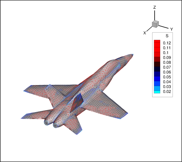
The mesh plot layer displays the lines connecting neighboring data points within a Zone. For I-ordered data, the mesh is a single line connecting all of the points in order of increasing I-index. For IJ-ordered data, the mesh consists of two families of lines connecting adjacent data points of increasing I-index and increasing J-index. For IJK-ordered data, the mesh consists of three families of lines, one connecting points of increasing I-index, one connecting points of increasing J-index, and one connecting points of increasing K-index. For finite element zones, the mesh is a plot of every edge of all of the elements that are defined by the connectivity list for the node points:

from os import path
import numpy as np
import tecplot as tp
from tecplot.constant import PlotType, MeshType

examples_dir = tp.session.tecplot_examples_directory()
infile = path.join(examples_dir, 'SimpleData', 'F18.plt')
dataset = tp.data.load_tecplot(infile)

# Enable 3D field plot and turn on contouring
frame = tp.active_frame()
frame.plot_type = PlotType.Cartesian3D
plot = frame.plot()
plot.show_mesh = True

contour = plot.contour(0)
contour.variable = dataset.variable('S')
contour.colormap_name = 'Doppler'
contour.levels.reset_levels(np.linspace(0.02,0.12,11))

# set the mesh type and color for all zones
mesh = plot.fieldmaps().mesh
mesh.mesh_type = MeshType.HiddenLine
mesh.color = contour

# save image to file
tp.export.save_png('fieldmap_mesh.png', 600, supersample=3)

Attributes

`color`	The `Color` or `ContourGroup` for lines.
`line_pattern`	`LinePattern` type to use for mesh lines.
`line_thickness`	Thickness (`float`) of the drawn lines.
`mesh_type`	`MeshType` to show.
`pattern_length`	Length (`float`) of the pattern segment for non-solid lines.
`show`	Draw the mesh for this fieldmap.

FieldmapMesh.color¶

The Color or ContourGroup for lines.

FieldmapContour lines can be a solid color or be colored by a ContourGroup as obtained through the plot.contour property. Note that changing style on this ContourGroup will affect all other fieldmaps on the same Frame that use it. Example usage:

>>> from tecplot.constant import Color
>>> plot.fieldmap(1).mesh.color = Color.Blue

Example of setting the color from a ContourGroup:

>>> plot.fieldmap(1).mesh.color = plot.contour(1)

Type:: Color or ContourGroup

FieldmapMesh.line_pattern¶

LinePattern type to use for mesh lines.

Possible values: Solid, Dashed, DashDot, Dotted, LongDash, DashDotDot.

Example usage:

>>> from tecplot.constant import LinePattern
>>> mesh = plot.fieldmap(0).mesh
>>> mesh.line_pattern = LinePattern.Dashed

Type:: LinePattern

FieldmapMesh.line_thickness¶

Thickness (float) of the drawn lines.

This is the line thickness in percentage of the Frame’s height. Example usage:

>>> plot.fieldmap(0).mesh.line_thickness = 0.7

Type:: float

FieldmapMesh.mesh_type¶

MeshType to show.

Possible values:

Wireframe

Wire frame meshes are drawn below any other zone layers on the same zone. In 3D Cartesian plots, no hidden lines are removed. For 3D volume zones (finite element volume or IJK-ordered), the full 3D mesh (consisting of all the connecting lines between data points) is not generally drawn because the sheer number of lines would make it confusing. The mesh drawn will depend on FieldmapSurfaces which can be obtained through the parent fieldmap with mesh.fieldmap.surfaces:

from tecplot.constant import MeshType, SurfacesToPlot
mesh = plot.fieldmap(0).mesh
mesh.mesh_type = MeshType.Wireframe
surfaces = mesh.fieldmap.surfaces
surfaces.surfaces_to_plot = SurfacesToPlot.IPlanes

By default, only the mesh on exposed cell faces is shown.

Overlay

Similar to Wire Frame, mesh lines are drawn over all other zone layers except for vectors and scatter symbols. In 3D Cartesian plots, the area behind the cells of the plot is still visible (unless another plot type such as contour flooding prevents this). As with Wire Frame, the mesh drawn will depend on FieldmapSurfaces which can be obtained through the parent fieldmap with mesh.fieldmap.surfaces.

HiddenLine

Similar to Overlay, except hidden lines are removed from behind the mesh. In effect, the cells (elements) of the mesh are opaque. FieldmapSurfaces and lines that are hidden behind another surface are removed from the plot. For 3D volume zones, using this plot type obscures everything inside the zone. If you choose this option for 3D volume zones, then choosing to plot every surface with:

from tecplot.constant import HiddenLine, SurfacesToPlot
mesh = plot.fieldmap(0).mesh
mesh.mesh_type = MeshType.HiddenLine
surfaces = mesh.fieldmap.surfaces
surfaces.surfaces_to_plot = SurfacesToPlot.All

has the same effect as plotting only exposed cell faces with:

surfaces.surfaces_to_plot = SurfacesToPlot.ExposedCellFaces

but is much slower.

Type:: MeshType

FieldmapMesh.pattern_length¶

Length (float) of the pattern segment for non-solid lines.

This is the pattern length in percentage of the Frame’s height. Example usage:

>>> plot.fieldmap(0).mesh.pattern_length = 3.5

Type:: float

FieldmapMesh.show¶

Draw the mesh for this fieldmap.

Example usage:

>>> from tecplot.constant import SurfacesToPlot
>>> plot.show_mesh = True
>>> surfaces = plot.fieldmap(0).surfaces
>>> surfaces.surfaces_to_plot = SurfacesToPlot.IPlanes
>>> plot.fieldmap(0).mesh.show = True

Type:: bool

FieldmapPoints ¶

class tecplot.plot.FieldmapPoints(fieldmap)[source]¶

Type and density of the points used for vector and scatter plots.

This object controls the location of the points for FieldmapVector and FieldmapScatter plots relative to the cells:

from os import path
import tecplot as tp
from tecplot.constant import PlotType, PointsToPlot

examples_dir = tp.session.tecplot_examples_directory()
infile = path.join(examples_dir, 'SimpleData', 'HeatExchanger.plt')
dataset = tp.data.load_tecplot(infile)

# Enable 3D field plot and turn on contouring
frame = tp.active_frame()
frame.plot_type = PlotType.Cartesian2D
plot = frame.plot()
plot.vector.u_variable = dataset.variable('U(M/S)')
plot.vector.v_variable = dataset.variable('V(M/S)')
plot.show_vector = True

points = plot.fieldmaps().points
points.points_to_plot = PointsToPlot.SurfaceCellCenters
points.step = (2,2)

# save image to file
tp.export.save_png('fieldmap_points.png', 600, supersample=3)

Attributes

`points_to_plot`	Location of the points to show.
`step`	Step along the dimensions `(I, J, K)`.

FieldmapPoints.points_to_plot¶

Location of the points to show.

Possible values:

SurfaceNodes: Draws only the nodes that are on the surface of the Zone.
AllNodes: Draws all nodes in the Zone.
SurfaceCellCenters: Draws points at the cell centers which are on or near the surface of the Zone.
AllCellCenters: Draws points at all cell centers in the Zone.
AllConnected: Draws all the nodes that are connected by the node map. Nodes without any connectivity are not drawn.

Example usage:

>>> from tecplot.constant import PointsToPlot
>>> pts = plot.fieldmap(0).points
>>> sts.points_to_plot = PointsToPlot.SurfaceCellCenters

Type:: PointsToPlot

FieldmapPoints.step¶

Step along the dimensions (I, J, K).

This property specifies the I, J, and K-step intervals. For irregular and finite element data, only the first parameter or I-Step has an effect. This steps through the nodes in the order they are listed in the data file. In this case, a single number can be given, but note that the return type is always a 3-tuple for both ordered and irregular data.

Example for IJK ordered data:

>>> plot.fieldmap(0).points.step = (10,10,None)
>>> print(plot.fieldmap(0).points.step)
(10, 10, 1)

Example for irregular data:

>>> plot.fieldmap(0).points.step = 10
>>> print(plot.fieldmap(0).points.step)
(10, 1, 1)

Type:: tuple

FieldmapScatter ¶

class tecplot.plot.FieldmapScatter(fieldmap)[source]¶

Plot of nodes using symbols.

FieldmapScatter plots display symbols at the data points in a field. The symbols may be sized according to the values of a specified variable, colored by the values of the contour variable, or may be uniformly sized or colored. Unlike contour plots, scatter plots do not require any mesh structure connecting the points, allowing scatter plots of irregular data:

from os import path
import tecplot as tp
from tecplot.constant import PlotType, SymbolType, FillMode

examples_dir = tp.session.tecplot_examples_directory()
infile = path.join(examples_dir, 'SimpleData', 'HeatExchanger.plt')
dataset = tp.data.load_tecplot(infile)

frame = tp.active_frame()
frame.plot_type = PlotType.Cartesian2D
plot = frame.plot()
plot.show_scatter = True

scatter = plot.fieldmaps().scatter
scatter.symbol_type = SymbolType.Geometry
scatter.fill_mode = FillMode.UseSpecificColor
scatter.fill_color = plot.contour(0)
scatter.size = 1

# ensure consistent output between interactive (connected) and batch
plot.contour(0).levels.reset_to_nice()

tp.export.save_png('fieldmap_scatter.png', 600, supersample=3)

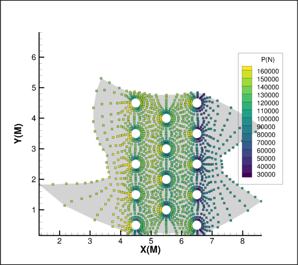
Attributes

`color`	Line `Color` or `ContourGroup` of the drawn symbols.
`fill_color`	Fill or background color.
`fill_mode`	Mode for the background color.
`line_thickness`	Width of the lines when drawing symbols.
`show`	Show the scatter symbols.
`size`	Size of the symbols to draw.
`size_by_variable`	Use a variable to determine relative size of symbols.
`symbol_type`	The `SymbolType` to use for this scatter plot.

Methods

symbol([symbol_type])

Returns a scatter symbol style object.

FieldmapScatter.color¶

Line Color or ContourGroup of the drawn symbols.

This can be a solid color or a ContourGroup as obtained through the plot.contour property. Note that changing style on the ContourGroup will affect all other fieldmaps in the same Frame that use it. Example usage:

>>> from tecplot.constant import Color
>>> plot.fieldmap(1).scatter.color = Color.Blue

Example of setting the color from a ContourGroup:

>>> plot.fieldmap(1).scatter.color = plot.contour(1)

Type:: Color or ContourGroup

FieldmapScatter.fill_color¶

Fill or background color.

The fill_mode attribute must be set accordingly:

>>> from tecplot.constant import Color, SymbolType, FillMode
>>> scatter = plot.fieldmap(0).scatter
>>> scatter.symbol_type = SymbolType.Geometry
>>> scatter.fill_mode = FillMode.UseSpecificColor
>>> scatter.fill_color = Color.Red

Type:: Color or ContourGroup

FieldmapScatter.fill_mode¶

Mode for the background color.

Options include: FillMode.UseSpecificColor, FillMode.UseLineColor, FillMode.UseBackgroundColor and FillMode.None_.

Example usage:

>>> from tecplot.constant import Color, SymbolType, FillMode
>>> scatter = plot.fieldmap(0).scatter
>>> scatter.symbol_type = SymbolType.Geometry
>>> scatter.fill_mode = FillMode.UseSpecificColor
>>> scatter.fill_color = Color.Red

Type:: FillMode

FieldmapScatter.line_thickness¶

Width of the lines when drawing symbols.

Example usage:

>>> from tecplot.constant import SymbolType
>>> scatter = plot.fieldmap(0).scatter
>>> scatter.symbol_type = SymbolType.Geometry
>>> scatter.line_thickness = 1

Type:: float

FieldmapScatter.show¶

Show the scatter symbols.

Example usage:

>>> plot.show_scatter = True
>>> plot.fieldmap(2).scatter.show = True

Type:: bool

FieldmapScatter.size¶

Size of the symbols to draw.

Example usage:

>>> plot.fieldmap(0).scatter.size = 4

Type:: float

FieldmapScatter.size_by_variable¶

Use a variable to determine relative size of symbols.

Example usage:

>>> plot.scatter.variable = dataset.variable('P')
>>> plot.fieldmap(0).scatter.size_by_variable = True

See also

Scatter.variable

Type:: bool

FieldmapScatter.symbol(symbol_type=None)[source]¶

Returns a scatter symbol style object.

Parameters:: symbol_type (SymbolType, optional) – The type of symbol to return. By default, this will return the active symbol type which is obtained from FieldmapScatter.symbol_type.

Returns: TextScatterSymbol or GeometryScatterSymbol

Example usage:

>>> from tecplot.constant import SymbolType
>>> plot.fieldmap(0).scatter.symbol_type = SymbolType.Text
>>> symbol = plot.fieldmap(0).scatter.symbol()
>>> symbol.text = 'a'

FieldmapScatter.symbol_type¶

The SymbolType to use for this scatter plot.

Possible values are SymbolType.Geometry or SymbolType.Text. Example usage:

>>> from tecplot.constant import SymbolType
>>> plot.fieldmap(0).scatter.symbol_type = SymbolType.Text

Type:: SymbolType

GeometryScatterSymbol ¶

class tecplot.plot.GeometryScatterSymbol(parent, svarg='SYMBOLSHAPE')[source]¶

Geometric shape for scatter plots.

from os import path
import tecplot as tp
from tecplot.constant import (Color, PlotType, PointsToPlot, SymbolType,
                              GeomShape, FillMode)

examples_dir = tp.session.tecplot_examples_directory()
infile = path.join(examples_dir, 'SimpleData', 'HeatExchanger.plt')
dataset = tp.data.load_tecplot(infile)

frame = tp.active_frame()
frame.plot_type = PlotType.Cartesian2D
plot = frame.plot()
plot.show_scatter = True

# get handle to a collection of all fieldmaps
fmaps = plot.fieldmaps()

points = fmaps.points
points.points_to_plot = PointsToPlot.SurfaceCellCenters
points.step = (2,2)

scatter = fmaps.scatter
scatter.fill_mode = FillMode.UseSpecificColor
scatter.size = 2
scatter.line_thickness = 0.5
scatter.symbol_type = SymbolType.Geometry

for i, fmap in enumerate(fmaps):
    fmap.scatter.symbol().shape = GeomShape(i%7)
    fmap.scatter.color = Color(i)
    fmap.scatter.fill_color = Color(i + plot.num_fieldmaps)

tp.export.save_png('fieldmap_scatter_geometry.png', 600, supersample=3)

../_images/fieldmap_scatter_geometry.png

Attributes

shape

Geometric shape to use when plotting scatter points.

GeometryScatterSymbol.shape¶

Geometric shape to use when plotting scatter points.

Possible values: Square, Del, Grad, RTri, LTri, Diamond, Circle, Cube, Sphere, Octahedron, Point.

Example usage:

>>> from tecplot.constant import SymbolType, GeomShape
>>> scatter = plot.fieldmap(0).scatter
>>> scatter.symbol_type = SymbolType.Geometry
>>> scatter.symbol().shape = GeomShape.Diamond

Type:: GeomShape

TextScatterSymbol ¶

class tecplot.plot.TextScatterSymbol(parent, svarg='SYMBOLSHAPE')[source]¶

Text character for scatter plots.

Only a single character can be used.

from os import path
import tecplot as tp
from tecplot.constant import (Color, PlotType, PointsToPlot, SymbolType,
                                  GeomShape, FillMode)

examples_dir = tp.session.tecplot_examples_directory()
infile = path.join(examples_dir, 'SimpleData', 'HeatExchanger.plt')
dataset = tp.data.load_tecplot(infile)

frame = tp.active_frame()
frame.plot_type = PlotType.Cartesian2D
plot = frame.plot()
plot.show_shade = True
plot.show_scatter = True

# get handle to a collection of all fieldmaps
fmaps = plot.fieldmaps()

fmaps.points.points_to_plot = PointsToPlot.SurfaceCellCenters
fmaps.points.step = (4,4)
fmaps.shade.color = Color.LightBlue

fmaps.scatter.fill_mode = FillMode.UseSpecificColor
fmaps.scatter.fill_color = Color.Yellow
fmaps.scatter.size = 3
fmaps.scatter.symbol_type = SymbolType.Text

for i, fmap in enumerate(fmaps):
    fmap.scatter.color = Color((i % 4) + 13)
    fmap.scatter.symbol().text = hex(i)[-1]

tp.export.save_png('fieldmap_scatter_text.png', 600, supersample=3)

Attributes

`font_override`	Typeface to use when rendering text-based scatter.
`text`	The ASCII character to use as the symbol to show
`use_base_font`	Use the base typeface when rendering text-based scatter.

TextScatterSymbol.font_override¶

Typeface to use when rendering text-based scatter.

Possible values: constant.Font.Greek, constant.Font.Math or constant.Font.UserDefined.

The use_base_font attribute must be set to False:

>>> from tecplot.constant import SymbolType, Font
>>> scatter = plot.fieldmap(0).scatter
>>> scatter.symbol_type = SymbolType.Text
>>> scatter.symbol().use_base_font = False
>>> scatter.symbol().font_override = Font.Math

Type:: constant.Font

TextScatterSymbol.text¶

The ASCII character to use as the symbol to show

Note

This is limited to a single character.

Example usage:

>>> from tecplot.constant import SymbolType
>>> scatter = plot.fieldmap(0).scatter
>>> scatter.symbol_type = SymbolType.Text
>>> scatter.symbol().text = 'X'

TextScatterSymbol.use_base_font¶

Use the base typeface when rendering text-based scatter.

When False, the font_override attribute takes effect:

>>> from tecplot.constant import SymbolType, Font
>>> scatter = plot.fieldmap(0).scatter
>>> scatter.symbol_type = SymbolType.Text
>>> scatter.symbol().use_base_font = False
>>> scatter.symbol().font_override = Font.Greek

Type:: bool

FieldmapShade ¶

class tecplot.plot.FieldmapShade(fieldmap)[source]¶

Fill color for displayed surfaces on 2D field plots.

Although most commonly used with 3D surfaces (see FieldmapShade3D), shade plots can be used to flood 2D plots with solid colors.

import os
import random
import tecplot
from tecplot.constant import Color, PlotType

random.seed(1)

examples_dir = tecplot.session.tecplot_examples_directory()
datafile = os.path.join(examples_dir, 'SimpleData', 'F18.plt')
dataset = tecplot.data.load_tecplot(datafile)
frame = dataset.frame
frame.plot_type = PlotType.Cartesian2D
plot = frame.plot()

for zone in dataset.zones():
    color = Color(random.randint(0,63))
    while color == Color.White:
        color = Color(random.randint(0,63))
    plot.fieldmap(zone).shade.color = color

tecplot.export.save_png('fieldmap_shade2d.png', 600, supersample=3)

Attributes

`color`	Fill `Color` of the shade.
`show`	FieldmapShade the drawn surfaces.

FieldmapShade.color¶

Fill Color of the shade.

Example usage:

>>> from tecplot.constant import Color
>>> plot.fieldmap(0).shade.color = Color.Blue

Type:: Color

FieldmapShade.show¶

FieldmapShade the drawn surfaces.

Example usage:

>>> plot.fieldmap(0).shade.show = False

Type:: bool

FieldmapShade3D ¶

class tecplot.plot.FieldmapShade3D(fieldmap)[source]¶

Fill color for displayed surfaces on 3D field plots.

This class inherits all functionality and purpose from FieldmapShade and adds the ability to turn on or off the lighting effect. In 3D plots, fieldmap effects (translucency and lighting) cause color variation (shading) throughout the zones. Shading can can be useful in discerning the shape of the data:

import os
import random
import tecplot
from tecplot.constant import Color, PlotType, SurfacesToPlot

random.seed(1)

examples_dir = tecplot.session.tecplot_examples_directory()
datafile = os.path.join(examples_dir, 'SimpleData', 'F18.plt')
dataset = tecplot.data.load_tecplot(datafile)
frame = dataset.frame
frame.plot_type = PlotType.Cartesian3D
plot = frame.plot()

for zone in dataset.zones():
    color = Color(random.randint(0,63))
    while color == Color.White:
        color = Color(random.randint(0,63))
    fmap = plot.fieldmap(zone)
    fmap.surfaces.surfaces_to_plot = SurfacesToPlot.BoundaryFaces
    fmap.shade.color = color
    fmap.shade.use_lighting_effect = False

tecplot.export.save_png('fieldmap_shade3d.png', 600, supersample=3)

Attributes

`color`	Fill `Color` of the shade.
`show`	FieldmapShade the drawn surfaces.
`use_lighting_effect`	Draw a lighting effect on the shaded surfaces.

FieldmapShade3D.color¶

Fill Color of the shade.

Example usage:

>>> from tecplot.constant import Color
>>> plot.fieldmap(0).shade.color = Color.Blue

Type:: Color

FieldmapShade3D.show¶

FieldmapShade the drawn surfaces.

Example usage:

>>> plot.fieldmap(0).shade.show = False

Type:: bool

FieldmapShade3D.use_lighting_effect¶

Draw a lighting effect on the shaded surfaces.

Example usage:

>>> plot.fieldmap(0).shade.use_lighting_effect = False

Type:: bool

FieldmapSurfaces ¶

class tecplot.plot.FieldmapSurfaces(fieldmap)[source]¶

Plot surfaces from volume data.

This class controls viewing volume data as surfaces, either via a boundary surface or one or more planes along the I, J, K dimensions for ordered data:

import numpy as np

import tecplot as tp
from tecplot.constant import *
from tecplot.data.operate import execute_equation

# Get the active frame, setup a grid (30x30x30)
# where each dimension ranges from 0 to 30.
# Add variable P to the dataset and give
# values to the data.
frame = tp.active_frame()
dataset = frame.dataset
for v in ['X','Y','Z','P']:
    dataset.add_variable(v)
zone = dataset.add_ordered_zone('Zone', (30,30,30))
xx = np.linspace(0,30,30)
for v,arr in zip(['X','Y','Z'],np.meshgrid(xx,xx,xx)):
    zone.values(v)[:] = arr.ravel()
execute_equation('{P} = -10*{X} + {Y}**2 + {Z}**2')

# Enable 3D field plot and turn on contouring
frame.plot_type = PlotType.Cartesian3D
plot = frame.plot()
plot.show_contour = True

# get a handle of the fieldmap for this zone
fmap = plot.fieldmap(dataset.zone('Zone'))

# set the active contour group to flood by variable P
fmap.contour.flood_contour_group.variable = dataset.variable('P')
plot.contour(0).levels.reset_to_nice()

# show I and J-planes through the surface
fmap.surfaces.surfaces_to_plot = SurfacesToPlot.IJPlanes

# show only the first and last I-planes
# min defaults to 0, max defaults to -1
# we set step to -1 which is equivalent
# to the I-dimensions's max
fmap.surfaces.i_range = None,None,-1

# show J-planes at indices: [5, 15, 25]
fmap.surfaces.j_range = 5,25,10

# save image to file
tp.export.save_png('fieldmap_surfaces_ij.png', 600, supersample=3)

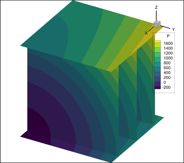
Attributes

`i_range`	`IndexRange` for the I dimension of ordered data.
`j_range`	`IndexRange` for the J dimension of ordered data.
`k_range`	`IndexRange` for the K dimension of ordered data.
`surfaces_to_plot`	The surfaces to show.

FieldmapSurfaces.i_range¶

IndexRange for the I dimension of ordered data.

This example shows I-planes at i = [0, 2, 4, 6, 8, 10]:

>>> from tecplot.constant import SurfacesToPlot
>>> srf = frame.plot().fieldmap(0).surfaces
>>> srf.surfaces_to_plot = SurfacesToPlot.IPlanes
>>> srf.i_range = 0, 10, 2

Type:: tuple of integers (min, max, step)

FieldmapSurfaces.j_range¶

IndexRange for the J dimension of ordered data.

This example shows all J-planes starting with j = 10 up to the maximum J-plane of the associated Zone:

>>> from tecplot.constant import SurfacesToPlot
>>> srf = frame.plot().fieldmap(0).surfaces
>>> srf.surfaces_to_plot = SurfacesToPlot.JPlanes
>>> srf.j_range = 10, None, 1

Type:: tuple of integers (min, max, step)

FieldmapSurfaces.k_range¶

IndexRange for the K dimension of ordered data.

This example shows all K-planes starting with the first up to 5 from the last K-plane of the associated Zone:

>>> from tecplot.constant import SurfacesToPlot
>>> srf = frame.plot().fieldmap(0).surfaces
>>> srf.surfaces_to_plot = SurfacesToPlot.KPlanes
>>> srf.k_range = None, -5

Type:: tuple of integers (min, max, step)

FieldmapSurfaces.surfaces_to_plot¶

The surfaces to show.

Possible values: BoundaryFaces, ExposedCellFaces, IPlanes, JPlanes, KPlanes, IJPlanes, JKPlanes, IKPlanes, IJKPlanes, All, the python built-in None.

Options such as IJKPlanes show planes from multiple dimensions. For example, the IJPlanes value shows both the I-planes and the J-planes. The following example shows a 3D field plot using faces on the boundary:

>>> from tecplot.constant import SurfacesToPlot
>>> frame.plot_type = PlotType.Cartesian3D
>>> srf = frame.plot().fieldmap(0).surfaces
>>> srf.surfaces_to_plot = SurfacesToPlot.BoundaryFaces

Type:: SurfacesToPlot

FieldmapVector ¶

class tecplot.plot.FieldmapVector(fieldmap)[source]¶

Field plot of arrows.

Before doing anything with vector plots, one must set the variables to be used for the (U, V, W) coordinates. This is done through the plot object. Once set, the vectors can be displayed and manipulated using this class:

import numpy as np
import tecplot as tp
from tecplot.data.operate import execute_equation
from tecplot.constant import (PlotType, PointsToPlot, VectorType,
                              ArrowheadStyle)

frame = tp.active_frame()
dataset = frame.dataset
for v in ['X','Y','Z','P','Q','R']:
    dataset.add_variable(v)
zone = dataset.add_ordered_zone('Zone', (30,30,30))
xx = np.linspace(0,30,30)
for v,arr in zip(['X','Y','Z'],np.meshgrid(xx,xx,xx)):
    zone.values(v)[:] = arr.ravel()
execute_equation('{P} = -10 * {X}    +      {Y}**2 + {Z}**2')
execute_equation('{Q} =       {X}    - 10 * {Y}    - {Z}**2')
execute_equation('{R} =       {X}**2 +      {Y}**2 - {Z}   ')

frame.plot_type = PlotType.Cartesian3D
plot = frame.plot()
plot.contour(0).variable = dataset.variable('P')
plot.contour(0).colormap_name = 'Two Color'
plot.contour(0).levels.reset_to_nice()
plot.vector.u_variable = dataset.variable('P')
plot.vector.v_variable = dataset.variable('Q')
plot.vector.w_variable = dataset.variable('R')
plot.show_vector = True

points = plot.fieldmap(0).points
points.points_to_plot = PointsToPlot.AllNodes
points.step = (5,3,2)

vector = plot.fieldmap(0).vector
vector.show = True
vector.vector_type = VectorType.MidAtPoint
vector.arrowhead_style = ArrowheadStyle.Filled
vector.color = plot.contour(0)
vector.line_thickness = 0.4

# save image to file
tp.export.save_png('fieldmap_vector.png', 600, supersample=3)

Attributes

`arrowhead_style`	The `ArrowheadStyle` drawn.
`color`	The `Color` or `ContourGroup` to use when drawing vectors.
`line_pattern`	The `LinePattern` used to draw the arrow line.
`line_thickness`	The width of the arrow line.
`pattern_length`	Length of the pattern used when drawing vector lines.
`show`	Enable drawing vectors on the plot.
`tangent_only`	Show only tangent vectors.
`vector_type`	Anchor point of the drawn vectors.

FieldmapVector.arrowhead_style¶

The ArrowheadStyle drawn.

Possible values: Plain, Filled, Hollow.

Example usage:

>>> from tecplot.constant import ArrowheadStyle
>>> plot.fieldmap(0).vector.arrowhead_style = ArrowheadStyle.Filled

Type:: ArrowheadStyle

FieldmapVector.color¶

The Color or ContourGroup to use when drawing vectors.

FieldmapVectors can be a solid color or be colored by a ContourGroup as obtained through the plot.contour property. Note that changing style on this ContourGroup will affect all other fieldmaps on the same Frame that use it. Example usage:

>>> from tecplot.constant import Color
>>> plot.fieldmap(1).vector.color = Color.Blue

Example of setting the color from a ContourGroup:

>>> plot.fieldmap(1).vector.color = plot.contour(1)

Type:: Color or ContourGroup

FieldmapVector.line_pattern¶

The LinePattern used to draw the arrow line.

Possible values: Solid, Dashed, DashDot, Dotted, LongDash, DashDotDot.

Example usage:

>>> from tecplot.constant import LinePattern
>>> vector = plot.fieldmap(0).vector
>>> vector.line_pattern = LinePattern.DashDot

Type:: LinePattern

FieldmapVector.line_thickness¶

The width of the arrow line.

Example usage:

>>> from tecplot.constant import LinePattern
>>> vector = plot.fieldmap(0).vector.line_thickness = 0.7

Type:: float (percentage of Frame height)

FieldmapVector.pattern_length¶

Length of the pattern used when drawing vector lines.

Example usage:

>>> from tecplot.constant import LinePattern
>>> vector = plot.fieldmap(0).vector
>>> vector.line_pattern = LinePattern.Dashed
>>> vector.pattern_length = 3.5

Type:: float (percentage of Frame height)

FieldmapVector.show¶

Enable drawing vectors on the plot.

Example usage:

>>> plot.show_vector = True
>>> plot.fieldmap(0).vector.show = True

Type:: bool

FieldmapVector.tangent_only¶

Show only tangent vectors.

Set to True to display only the tangent component of vectors. Tangent vectors are drawn on 3D surfaces only where it is possible to determine a vector normal to the surface. A plot where multiple surfaces intersect each other using common nodes is a case where tangent vectors are not drawn because there is more than one normal to choose from. An example of this would be a volume IJK-ordered zone where both the I and J-planes are shown. If tangent vectors cannot be drawn, then regular vectors are plotted instead.

Example usage:

>>> plot.fieldmap(0).vector.tangent_only = True

Type:: bool

FieldmapVector.vector_type¶

Anchor point of the drawn vectors.

Possible values: TailAtPoint, HeadAtPoint, MidAtPoint, HeadOnly.

Example usage:

>>> from tecplot.constant import VectorType
>>> plot.fieldmap(0).vector.vector_type = VectorType.MidAtPoint

Type:: VectorType

Linemaps ¶

PolarLinemap ¶

class tecplot.plot.PolarLinemap(plot, *indices)[source]¶

Data mapping and style control for polar line plots.

Attributes

`aux_data`	Auxiliary data for this linemap.
`curve`	Style and fitting-method control for lines.
`function_dependency`	The independent variable for function evalulation.
`index`	Zero-based integer identifier for this Linemaps.
`indices`	Object controlling which lines are shown.
`line`	Style for lines to be drawn.
`linemap_indices`	Read-only, sorted `list` of zero-based fieldmap indices.
`name`	Name identifier of this Linemaps.
`r_axis`	Radial axis used by this linemap.
`r_variable`	\(r\)-component `Variable` of the plotted line.
`r_variable_index`	\(r\)-component `Variable` index of the plotted line.
`show`	Display this linemap on the plot.
`show_in_legend`	Show this Linemaps in the legend.
`sort_mode`	Control which `Variable` to use when sorting lines.
`sort_variable`	Specific `Variable` used when listing lines.
`sort_variable_index`	Zero-based index of the specific `Variable` used for sorting.
`symbols`	Style for markers at points along the lines.
`theta_axis`	Angular axis used by this linemap.
`theta_variable`	:math:` heta`-component `Variable` of the plotted line.
`theta_variable_index`	:math:` heta`-component `Variable` index of the plotted line.
`zone`	Data source (Zone) for this Linemaps.
`zone_index`	Zero-based index of the Zone this Linemaps will draw.

PolarLinemap.aux_data¶

Auxiliary data for this linemap.

Returns: AuxData

This is the auxiliary data attached to the linemap. Such data is written to the layout file by default and can be retrieved later. Example usage:

>>> from tecplot.constant import PlotType
>>> plot = tp.active_frame().plot(PlotType.XYLine)
>>> aux = plot.linemap(0).aux_data
>>> aux['Result'] = '3.14159'
>>> print(aux['Result'])
3.14159

PolarLinemap.curve¶

Style and fitting-method control for lines.

Type:: LinemapCurve

PolarLinemap.function_dependency¶

The independent variable for function evalulation.

Possible values: RIndependent, ThetaIndependent. Example usage:

>>> from tecplot.constant import FunctionDependency, PlotType
>>> plot = frame.plot(PlotType.PolarLine)
>>> lmap = plot.linemap(0)
>>> lmap.function_dependency = FunctionDependency.ThetaIndependent

Type:: FunctionDependency

PolarLinemap.index¶

Zero-based integer identifier for this Linemaps.

Example:

>>> lmap = plot.linemap(1)
>>> print(lmap.index)
1

Type:: int

PolarLinemap.indices¶

Object controlling which lines are shown.

Type:: LinemapIndices

PolarLinemap.line¶

Style for lines to be drawn.

Type:: LinemapLine

PolarLinemap.linemap_indices¶

Read-only, sorted list of zero-based fieldmap indices.

Type:: list

PolarLinemap.name¶

Name identifier of this Linemaps.

Names are automatically assigned to each mapping. The nature of the name depends on the type of data used to create the mapping. If your data has only one dependent variable, the default is to use the zone name for the mapping. If your data has multiple dependent variables, then the default is to use the dependent variable name for the mapping. In either case each mapping is assigned a special name (&ZN& or &DN&) that is replaced with the zone or variable name when the name is displayed.

Selecting variables in a 3D finite element zone may require significant time, since the variable must be loaded over the entire zone. XY and Polar line plots are best used with linear or ordered data, or with two-dimensional finite element data.

Certain placeholder text will be replaced with values based on elements within the plot. By combining static text with these placeholders, you can construct a name in any format you like:

>>> plot.linemap(2).name = 'Zone: &ZN&'

The placeholders available are:

Zone name (&ZN&): This will be replaced with the actual name of the zone assigned to that mapping.
Zone number (&Z#&): This will be replaced with the actual number of the zone assigned to the mapping.
Independent variable name (&IV&): This will be replaced with the actual name of the independent variable assigned to that mapping.
Independent variable number (&I#&): This will be replaced with the actual number of the independent variable assigned to the mapping.
Dependent variable name (&DV&): This will be replaced with the actual name of the dependent variable assigned to that mapping.
Dependent variable number (&D#&): This will be replaced with the actual number of the dependent variable assigned to the mapping.
Map number (&M#&): This will be replaced with the actual number of the mapping.
X-Axis number (&X#&): This will be replaced with the actual number of the X-axis assigned to that mapping for XY Line plots. This option is not available for Polar Line plots.
Y-Axis number (&Y#&): This will be replaced with the actual number of the Y-axis assigned to that mapping for XY Line plots. This option is not available for Polar Line plots.

Type:: str

PolarLinemap.r_axis¶

Radial axis used by this linemap.

Example usage:

>>> from tecplot.constant import PlotType
>>> plot = frame.plot(PlotType.PolarLine)
>>> plot.linemap(0).r_axis.title = 'distance (m)'

Type:: RadialLineAxis

PolarLinemap.r_variable¶

\(r\)-component Variable of the plotted line.

Example usage:

>>> from tecplot.constant import PlotType
>>> plot = frame.plot(PlotType.PolarLine)
>>> plot.linemap(0).r_variable = dataset.variable('R')

Type:: Variable

PolarLinemap.r_variable_index¶

\(r\)-component Variable index of the plotted line.

Example usage:

>>> from tecplot.constant import PlotType
>>> plot = frame.plot(PlotType.PolarLine)
>>> plot.linemap(0).r_variable_index = 0

Type:: int (Zero-based index)

PolarLinemap.show¶

Display this linemap on the plot.

Example usage for turning on all linemaps:

>>> for lmap in plot.linemaps():
...     lmap.show = True

Type:: bool

PolarLinemap.show_in_legend¶

Show this Linemaps in the legend.

Possible values:

LegendShow.Always: The mapping appears in the legend even if the mapping is turned off (deactivated) or its entry in the table looks exactly like another mapping’s entry.
LegendShow.Never: The mapping never appears in the legend.
LegendShow.Auto (default): The mapping appears in the legend only when the mapping is turned on. If two mappings would result in the same entry in the legend, only one entry is shown.

Type:: LegendShow

PolarLinemap.sort_mode¶

Control which Variable to use when sorting lines.

Possible values: LineMapSort.BySpecificVar, LineMapSort.ByIndependentVar, LineMapSort.ByDependentVar or LineMapSort.None_.

Example usage:

>>> from tecplot.constant import LineMapSort
>>> plot.linemap(0).sort_mode = LineMapSort.ByDependentVar

Type:: LineMapSort

PolarLinemap.sort_variable¶

Specific Variable used when listing lines.

The sort_mode attribute must be set to LineMapSort.BySpecificVar:

>>> from tecplot.constant import LineMapSort
>>> plot.linemap(0).sort_by = LineMapSort.BySpecificVar
>>> plot.linemap(0).sort_variable = dataset.variable('P')

Type:: Variable

PolarLinemap.sort_variable_index¶

Zero-based index of the specific Variable used for sorting.

The sort_mode attribute must be set to LineMapSort.BySpecificVar:

>>> from tecplot.constant import LineMapSort
>>> plot.linemap(0).sort_by = LineMapSort.BySpecificVar
>>> plot.linemap(0).sort_variable_index = 3

Type:: int

PolarLinemap.symbols¶

Style for markers at points along the lines.

Type:: LinemapSymbols

PolarLinemap.theta_axis¶

Angular axis used by this linemap.

Example usage:

>>> from tecplot.constant import PlotType
>>> plot = frame.plot(PlotType.PolarLine)
>>> plot.linemap(0).theta_axis.title = 'angle (deg)'

Type:: PolarAngleLineAxis

PolarLinemap.theta_variable¶

:math:` heta`-component Variable of the plotted line.

Example usage:

>>> from tecplot.constant import PlotType
>>> plot = frame.plot(PlotType.PolarLine)
>>> plot.linemap(0).theta_variable = dataset.variable('Theta')

Type:: Variable

PolarLinemap.theta_variable_index¶

:math:` heta`-component Variable index of the plotted line.

Example usage:

>>> from tecplot.constant import PlotType
>>> plot = frame.plot(PlotType.PolarLine)
>>> plot.linemap(0).theta_variable_index = 1

Type:: int (Zero-based index)

PolarLinemap.zone¶

Data source (Zone) for this Linemaps.

Example usage:

>>> plot.linemap(0).zone = dataset.zone('Zone 1')

PolarLinemap.zone_index¶

Zero-based index of the Zone this Linemaps will draw.

Example usage:

>>> plot.linemap(0).zone_index = 2

Type:: int

PolarLinemapCollection ¶

class tecplot.plot.PolarLinemapCollection(plot, *indices)[source]¶

Data mapping and style control for one or more polar line plots.

New in version 1.1: Linemap collection objects.

Attributes

`curve`	Style and fitting-method control for lines.
`function_dependency`	The independent variable for function evalulation.
`indices`	Object controlling which lines are shown.
`line`	Style for lines to be drawn.
`linemap_indices`	Read-only, sorted `list` of zero-based fieldmap indices.
`name`	Name identifier of this Linemaps.
`r_axis`	Radial axis used by this linemap.
`r_variable`	\(r\)-component `Variable` of the plotted line.
`r_variable_index`	\(r\)-component `Variable` index of the plotted line.
`show`	Display this linemap on the plot.
`show_in_legend`	Show this Linemaps in the legend.
`sort_mode`	Control which `Variable` to use when sorting lines.
`sort_variable`	Specific `Variable` used when listing lines.
`sort_variable_index`	Zero-based index of the specific `Variable` used for sorting.
`symbols`	Style for markers at points along the lines.
`theta_axis`	Angular axis used by this linemap.
`theta_variable`	:math:` heta`-component `Variable` of the plotted line.
`theta_variable_index`	:math:` heta`-component `Variable` index of the plotted line.
`zone`	Zones of this LinemapCollection.
`zone_index`	Zero-based index of the Zone this Linemaps will draw.

PolarLinemapCollection.curve¶

Style and fitting-method control for lines.

Type:: LinemapCurve

PolarLinemapCollection.function_dependency¶

The independent variable for function evalulation.

Possible values: RIndependent, ThetaIndependent. Example usage:

>>> from tecplot.constant import FunctionDependency, PlotType
>>> plot = frame.plot(PlotType.PolarLine)
>>> lmap = plot.linemap(0)
>>> lmap.function_dependency = FunctionDependency.ThetaIndependent

Type:: FunctionDependency

PolarLinemapCollection.indices¶

Object controlling which lines are shown.

Type:: LinemapIndices

PolarLinemapCollection.line¶

Style for lines to be drawn.

Type:: LinemapLine

PolarLinemapCollection.linemap_indices¶

Read-only, sorted list of zero-based fieldmap indices.

Type:: list

PolarLinemapCollection.name¶

Name identifier of this Linemaps.

Names are automatically assigned to each mapping. The nature of the name depends on the type of data used to create the mapping. If your data has only one dependent variable, the default is to use the zone name for the mapping. If your data has multiple dependent variables, then the default is to use the dependent variable name for the mapping. In either case each mapping is assigned a special name (&ZN& or &DN&) that is replaced with the zone or variable name when the name is displayed.

Selecting variables in a 3D finite element zone may require significant time, since the variable must be loaded over the entire zone. XY and Polar line plots are best used with linear or ordered data, or with two-dimensional finite element data.

Certain placeholder text will be replaced with values based on elements within the plot. By combining static text with these placeholders, you can construct a name in any format you like:

>>> plot.linemap(2).name = 'Zone: &ZN&'

The placeholders available are:

Zone name (&ZN&): This will be replaced with the actual name of the zone assigned to that mapping.
Zone number (&Z#&): This will be replaced with the actual number of the zone assigned to the mapping.
Independent variable name (&IV&): This will be replaced with the actual name of the independent variable assigned to that mapping.
Independent variable number (&I#&): This will be replaced with the actual number of the independent variable assigned to the mapping.
Dependent variable name (&DV&): This will be replaced with the actual name of the dependent variable assigned to that mapping.
Dependent variable number (&D#&): This will be replaced with the actual number of the dependent variable assigned to the mapping.
Map number (&M#&): This will be replaced with the actual number of the mapping.
X-Axis number (&X#&): This will be replaced with the actual number of the X-axis assigned to that mapping for XY Line plots. This option is not available for Polar Line plots.
Y-Axis number (&Y#&): This will be replaced with the actual number of the Y-axis assigned to that mapping for XY Line plots. This option is not available for Polar Line plots.

Type:: str

PolarLinemapCollection.r_axis¶

Radial axis used by this linemap.

Example usage:

>>> from tecplot.constant import PlotType
>>> plot = frame.plot(PlotType.PolarLine)
>>> plot.linemap(0).r_axis.title = 'distance (m)'

Type:: RadialLineAxis

PolarLinemapCollection.r_variable¶

\(r\)-component Variable of the plotted line.

Example usage:

>>> from tecplot.constant import PlotType
>>> plot = frame.plot(PlotType.PolarLine)
>>> plot.linemap(0).r_variable = dataset.variable('R')

Type:: Variable

PolarLinemapCollection.r_variable_index¶

\(r\)-component Variable index of the plotted line.

Example usage:

>>> from tecplot.constant import PlotType
>>> plot = frame.plot(PlotType.PolarLine)
>>> plot.linemap(0).r_variable_index = 0

Type:: int (Zero-based index)

PolarLinemapCollection.show¶

Display this linemap on the plot.

Example usage for turning on all linemaps:

>>> plot.linemaps().show = True

Type:: bool

PolarLinemapCollection.show_in_legend¶

Show this Linemaps in the legend.

Possible values:

LegendShow.Always: The mapping appears in the legend even if the mapping is turned off (deactivated) or its entry in the table looks exactly like another mapping’s entry.
LegendShow.Never: The mapping never appears in the legend.
LegendShow.Auto (default): The mapping appears in the legend only when the mapping is turned on. If two mappings would result in the same entry in the legend, only one entry is shown.

Type:: LegendShow

PolarLinemapCollection.sort_mode¶

Control which Variable to use when sorting lines.

Possible values: LineMapSort.BySpecificVar, LineMapSort.ByIndependentVar, LineMapSort.ByDependentVar or LineMapSort.None_.

Example usage:

>>> from tecplot.constant import LineMapSort
>>> plot.linemap(0).sort_mode = LineMapSort.ByDependentVar

Type:: LineMapSort

PolarLinemapCollection.sort_variable¶

Specific Variable used when listing lines.

The sort_mode attribute must be set to LineMapSort.BySpecificVar:

>>> from tecplot.constant import LineMapSort
>>> plot.linemap(0).sort_by = LineMapSort.BySpecificVar
>>> plot.linemap(0).sort_variable = dataset.variable('P')

Type:: Variable

PolarLinemapCollection.sort_variable_index¶

Zero-based index of the specific Variable used for sorting.

The sort_mode attribute must be set to LineMapSort.BySpecificVar:

>>> from tecplot.constant import LineMapSort
>>> plot.linemap(0).sort_by = LineMapSort.BySpecificVar
>>> plot.linemap(0).sort_variable_index = 3

Type:: int

PolarLinemapCollection.symbols¶

Style for markers at points along the lines.

Type:: LinemapSymbols

PolarLinemapCollection.theta_axis¶

Angular axis used by this linemap.

Example usage:

>>> from tecplot.constant import PlotType
>>> plot = frame.plot(PlotType.PolarLine)
>>> plot.linemap(0).theta_axis.title = 'angle (deg)'

Type:: PolarAngleLineAxis

PolarLinemapCollection.theta_variable¶

:math:` heta`-component Variable of the plotted line.

Example usage:

>>> from tecplot.constant import PlotType
>>> plot = frame.plot(PlotType.PolarLine)
>>> plot.linemap(0).theta_variable = dataset.variable('Theta')

Type:: Variable

PolarLinemapCollection.theta_variable_index¶

:math:` heta`-component Variable index of the plotted line.

Example usage:

>>> from tecplot.constant import PlotType
>>> plot = frame.plot(PlotType.PolarLine)
>>> plot.linemap(0).theta_variable_index = 1

Type:: int (Zero-based index)

PolarLinemapCollection.zone¶

Zones of this LinemapCollection.

Example usage:

>>> print([z.name for z in plot.linemaps().zone])
['Zone 1', 'Zone 2']

New in version 1.6: Linemap collection zone property.

Type:: tuple of Zones

PolarLinemapCollection.zone_index¶

Zero-based index of the Zone this Linemaps will draw.

Example usage:

>>> plot.linemap(0).zone_index = 2

Type:: int

XYLinemap ¶

class tecplot.plot.XYLinemap(plot, *indices)[source]¶

Data mapping and style control for 2D Cartesian line plots.

Linemaps connect a specific Zone/Variable combination to a line or set of lines, depending on the dimension of the data if ordered. Linemaps can share any of the axes available in the plot and orientation can be verical or horizontal by setting the independent variable with XYLinemap.function_dependency:

from os import path
import tecplot as tp
from tecplot.constant import PlotType, Color

examples_dir = tp.session.tecplot_examples_directory()
infile = path.join(examples_dir, 'SimpleData', 'Rainfall.dat')
dataset = tp.data.load_tecplot(infile)

frame = tp.active_frame()
frame.plot_type = PlotType.XYLine
plot = frame.plot()

lmap = plot.linemap(0)
lmap.line.line_thickness = 0.8
lmap.line.color = Color.DeepRed
lmap.y_axis.title.color = Color.DeepRed

lmap = plot.linemap(1)
lmap.show = True
lmap.y_axis_index = 1
lmap.line.line_thickness = 0.8
lmap.line.color = Color.Blue
lmap.y_axis.title.color = lmap.line.color

tp.export.save_png('linemap_xy.png', 600, supersample=3)

See also

XYLinemapCollection

Attributes

`aux_data`	Auxiliary data for this linemap.
`bars`	`LinemapBars` style for bar charts.
`curve`	Style and fitting-method control for lines.
`error_bars`	`LinemapErrorBars` style for error bars.
`function_dependency`	The independent variable for function evalulation.
`index`	Zero-based integer identifier for this Linemaps.
`indices`	Object controlling which lines are shown.
`line`	Style for lines to be drawn.
`linemap_indices`	Read-only, sorted `list` of zero-based fieldmap indices.
`name`	Name identifier of this Linemaps.
`show`	Display this linemap on the plot.
`show_in_legend`	Show this Linemaps in the legend.
`sort_mode`	Control which `Variable` to use when sorting lines.
`sort_variable`	Specific `Variable` used when listing lines.
`sort_variable_index`	Zero-based index of the specific `Variable` used for sorting.
`symbols`	Style for markers at points along the lines.
`x_axis`	The X-axis used by this linemap.
`x_axis_index`	Zero-based index of the x-axis used by this linemap.
`x_variable`	`Variable` used for x-positions of this linemap.
`x_variable_index`	Zero-based index of the `Variable` used for x-positions.
`y_axis`	Y-axis used by this linemap.
`y_axis_index`	Zero-based index of the y-axis used by this linemap.
`y_variable`	`Variable` used for y-positions of this linemap.
`y_variable_index`	Zero-based index of the `Variable` used for y-positions.
`zone`	Data source (Zone) for this Linemaps.
`zone_index`	Zero-based index of the Zone this Linemaps will draw.

XYLinemap.aux_data¶

Auxiliary data for this linemap.

Returns: AuxData

This is the auxiliary data attached to the linemap. Such data is written to the layout file by default and can be retrieved later. Example usage:

>>> from tecplot.constant import PlotType
>>> plot = tp.active_frame().plot(PlotType.XYLine)
>>> aux = plot.linemap(0).aux_data
>>> aux['Result'] = '3.14159'
>>> print(aux['Result'])
3.14159

XYLinemap.bars¶

LinemapBars style for bar charts.

Type:: LinemapBars

XYLinemap.curve¶

Style and fitting-method control for lines.

Type:: LinemapCurve

XYLinemap.error_bars¶

LinemapErrorBars style for error bars.

Type:: LinemapErrorBars

XYLinemap.function_dependency¶

The independent variable for function evalulation.

Possible values: XIndependent, YIndependent.

Example usage:

>>> from tecplot.constant import FunctionDependency
>>> lmap = plot.linemap(0)
>>> lmap.function_dependency = FunctionDependency.YIndependent

Type:: FunctionDependency

XYLinemap.index¶

Zero-based integer identifier for this Linemaps.

Example:

>>> lmap = plot.linemap(1)
>>> print(lmap.index)
1

Type:: int

XYLinemap.indices¶

Object controlling which lines are shown.

Type:: LinemapIndices

XYLinemap.line¶

Style for lines to be drawn.

Type:: LinemapLine

XYLinemap.linemap_indices¶

Read-only, sorted list of zero-based fieldmap indices.

Type:: list

XYLinemap.name¶

Name identifier of this Linemaps.

Names are automatically assigned to each mapping. The nature of the name depends on the type of data used to create the mapping. If your data has only one dependent variable, the default is to use the zone name for the mapping. If your data has multiple dependent variables, then the default is to use the dependent variable name for the mapping. In either case each mapping is assigned a special name (&ZN& or &DN&) that is replaced with the zone or variable name when the name is displayed.

Selecting variables in a 3D finite element zone may require significant time, since the variable must be loaded over the entire zone. XY and Polar line plots are best used with linear or ordered data, or with two-dimensional finite element data.

Certain placeholder text will be replaced with values based on elements within the plot. By combining static text with these placeholders, you can construct a name in any format you like:

>>> plot.linemap(2).name = 'Zone: &ZN&'

The placeholders available are:

Zone name (&ZN&): This will be replaced with the actual name of the zone assigned to that mapping.
Zone number (&Z#&): This will be replaced with the actual number of the zone assigned to the mapping.
Independent variable name (&IV&): This will be replaced with the actual name of the independent variable assigned to that mapping.
Independent variable number (&I#&): This will be replaced with the actual number of the independent variable assigned to the mapping.
Dependent variable name (&DV&): This will be replaced with the actual name of the dependent variable assigned to that mapping.
Dependent variable number (&D#&): This will be replaced with the actual number of the dependent variable assigned to the mapping.
Map number (&M#&): This will be replaced with the actual number of the mapping.
X-Axis number (&X#&): This will be replaced with the actual number of the X-axis assigned to that mapping for XY Line plots. This option is not available for Polar Line plots.
Y-Axis number (&Y#&): This will be replaced with the actual number of the Y-axis assigned to that mapping for XY Line plots. This option is not available for Polar Line plots.

Type:: str

XYLinemap.show¶

Display this linemap on the plot.

Example usage for turning on all linemaps:

>>> for lmap in plot.linemaps():
...     lmap.show = True

Type:: bool

XYLinemap.show_in_legend¶

Show this Linemaps in the legend.

Possible values:

LegendShow.Always: The mapping appears in the legend even if the mapping is turned off (deactivated) or its entry in the table looks exactly like another mapping’s entry.
LegendShow.Never: The mapping never appears in the legend.
LegendShow.Auto (default): The mapping appears in the legend only when the mapping is turned on. If two mappings would result in the same entry in the legend, only one entry is shown.

Type:: LegendShow

XYLinemap.sort_mode¶

Control which Variable to use when sorting lines.

Possible values: LineMapSort.BySpecificVar, LineMapSort.ByIndependentVar, LineMapSort.ByDependentVar or LineMapSort.None_.

Example usage:

>>> from tecplot.constant import LineMapSort
>>> plot.linemap(0).sort_mode = LineMapSort.ByDependentVar

Type:: LineMapSort

XYLinemap.sort_variable¶

Specific Variable used when listing lines.

The sort_mode attribute must be set to LineMapSort.BySpecificVar:

>>> from tecplot.constant import LineMapSort
>>> plot.linemap(0).sort_by = LineMapSort.BySpecificVar
>>> plot.linemap(0).sort_variable = dataset.variable('P')

Type:: Variable

XYLinemap.sort_variable_index¶

Zero-based index of the specific Variable used for sorting.

The sort_mode attribute must be set to LineMapSort.BySpecificVar:

>>> from tecplot.constant import LineMapSort
>>> plot.linemap(0).sort_by = LineMapSort.BySpecificVar
>>> plot.linemap(0).sort_variable_index = 3

Type:: int

XYLinemap.symbols¶

Style for markers at points along the lines.

Type:: LinemapSymbols

XYLinemap.x_axis¶

The X-axis used by this linemap.

Example usage:

>>> plot.linemap(0).x_axis = plot.axes.x_axis(2)

Type:: XYLineAxis

XYLinemap.x_axis_index¶

Zero-based index of the x-axis used by this linemap.

Example usage:

>>> plot.linemap(0).x_axis_index = 2

Type:: int

XYLinemap.x_variable¶

Variable used for x-positions of this linemap.

Example usage:

>>> plot.linemap(0).x_variable = dataset.variable('P')

Type:: Variable

XYLinemap.x_variable_index¶

Zero-based index of the Variable used for x-positions.

Example usage:

>>> plot.linemap(0).x_variable_index = 2

Type:: int

XYLinemap.y_axis¶

Y-axis used by this linemap.

Example usage:

>>> plot.linemap(0).x_axis = plot.axes.y_axis(2)

Type:: XYLineAxis

XYLinemap.y_axis_index¶

Zero-based index of the y-axis used by this linemap.

Example usage:

>>> plot.linemap(0).y_axis_index = 2

Type:: int

XYLinemap.y_variable¶

Variable used for y-positions of this linemap.

Example usage:

>>> plot.linemap(0).y_variable = dataset.variable('Q')

Type:: Variable

XYLinemap.y_variable_index¶

Zero-based index of the Variable used for y-positions.

Example usage:

>>> plot.linemap(0).y_variable_index = 2

Type:: int

XYLinemap.zone¶

Data source (Zone) for this Linemaps.

Example usage:

>>> plot.linemap(0).zone = dataset.zone('Zone 1')

XYLinemap.zone_index¶

Zero-based index of the Zone this Linemaps will draw.

Example usage:

>>> plot.linemap(0).zone_index = 2

Type:: int

XYLinemapCollection ¶

class tecplot.plot.XYLinemapCollection(plot, *indices)[source]¶

Data mapping and style control for one or more line plots.

This class behaves like XYLinemap except that setting any underlying style will do so for all of the represented linemaps. The style properties are then always returned as a tuple of properties, one for each linemap, ordered by index number. This means there is an asymmetry between setting and getting any property under this object, illustrated by the following example:

>>> lmaps = plot.linemaps(0, 1, 2)
>>> lmaps.show = True
>>> print(lmaps.show)
(True, True, True)

This is the preferred way to control the style of many linemaps as it is much faster to execute. All examples that set style on a single linemap like the following:

>>> plot.linemap(0).line.color = Color.Blue

may be converted to setting the same style on all linemaps like so:

>>> plot.linemaps().line.color = Color.Blue

New in version 1.1: Linemap collection objects.

The Linemap layer controls how ordered or connected data is represented. This may be either a set of line segments connecting all the data points, or a curve fitted to the original data. This object represents one or more linemaps and can conveniently control the style for each one.

from os import path
import tecplot as tp
from tecplot.constant import PlotType, Color, LinePattern, AxisTitleMode

# load data from examples directory
examples_dir = tp.session.tecplot_examples_directory()
infile = path.join(examples_dir, 'SimpleData', 'Rainfall.dat')
dataset = tp.data.load_tecplot(infile)

# get handle to the active frame and set plot type to XY Line
frame = tp.active_frame()
frame.plot_type = PlotType.XYLine
plot = frame.plot()

# We will set the name, color and a few other properties
# for the first three linemaps in the dataset.
names = ['Seattle', 'Dallas', 'Miami']
colors = [Color.Blue, Color.DeepRed, Color.Khaki]

lmaps = plot.linemaps()

# set common style for all linemaps in the collection
lmaps.show = True
lmaps.line.line_thickness = 1
lmaps.line.line_pattern = LinePattern.LongDash
lmaps.line.pattern_length = 2

# loop over the linemaps, setting name and color for each
for lmap, name, color in zip(lmaps, names, colors):
    lmap.name = name
    lmap.line.color = color

# Set the y-axis label
plot.axes.y_axis(0).title.title_mode = AxisTitleMode.UseText
plot.axes.y_axis(0).title.text = 'Rainfall'

# Turn on legend
plot.legend.show = True

# Adjust the axes limits to show all the data
plot.view.fit()

# save image to file
tp.export.save_png('linemap.png', 600, supersample=3)

Attributes

`bars`	`LinemapBars` style for bar charts.
`curve`	Style and fitting-method control for lines.
`error_bars`	`LinemapErrorBars` style for error bars.
`function_dependency`	The independent variable for function evalulation.
`indices`	Object controlling which lines are shown.
`line`	Style for lines to be drawn.
`linemap_indices`	Read-only, sorted `list` of zero-based fieldmap indices.
`name`	Name identifier of this Linemaps.
`show`	Display this linemap on the plot.
`show_in_legend`	Show this Linemaps in the legend.
`sort_mode`	Control which `Variable` to use when sorting lines.
`sort_variable`	Specific `Variable` used when listing lines.
`sort_variable_index`	Zero-based index of the specific `Variable` used for sorting.
`symbols`	Style for markers at points along the lines.
`x_axis`	The X-axis used by this linemap.
`x_axis_index`	Zero-based index of the x-axis used by this linemap.
`x_variable`	`Variable` used for x-positions of this linemap.
`x_variable_index`	Zero-based index of the `Variable` used for x-positions.
`y_axis`	Y-axis used by this linemap.
`y_axis_index`	Zero-based index of the y-axis used by this linemap.
`y_variable`	`Variable` used for y-positions of this linemap.
`y_variable_index`	Zero-based index of the `Variable` used for y-positions.
`zone`	Zones of this LinemapCollection.
`zone_index`	Zero-based index of the Zone this Linemaps will draw.

XYLinemapCollection.bars¶

LinemapBars style for bar charts.

Type:: LinemapBars

XYLinemapCollection.curve¶

Style and fitting-method control for lines.

Type:: LinemapCurve

XYLinemapCollection.error_bars¶

LinemapErrorBars style for error bars.

Type:: LinemapErrorBars

XYLinemapCollection.function_dependency¶

The independent variable for function evalulation.

Possible values: XIndependent, YIndependent.

Example usage:

>>> from tecplot.constant import FunctionDependency
>>> lmap = plot.linemap(0)
>>> lmap.function_dependency = FunctionDependency.YIndependent

Type:: FunctionDependency

XYLinemapCollection.indices¶

Object controlling which lines are shown.

Type:: LinemapIndices

XYLinemapCollection.line¶

Style for lines to be drawn.

Type:: LinemapLine

XYLinemapCollection.linemap_indices¶

Read-only, sorted list of zero-based fieldmap indices.

Type:: list

XYLinemapCollection.name¶

Name identifier of this Linemaps.

Names are automatically assigned to each mapping. The nature of the name depends on the type of data used to create the mapping. If your data has only one dependent variable, the default is to use the zone name for the mapping. If your data has multiple dependent variables, then the default is to use the dependent variable name for the mapping. In either case each mapping is assigned a special name (&ZN& or &DN&) that is replaced with the zone or variable name when the name is displayed.

Selecting variables in a 3D finite element zone may require significant time, since the variable must be loaded over the entire zone. XY and Polar line plots are best used with linear or ordered data, or with two-dimensional finite element data.

Certain placeholder text will be replaced with values based on elements within the plot. By combining static text with these placeholders, you can construct a name in any format you like:

>>> plot.linemap(2).name = 'Zone: &ZN&'

The placeholders available are:

Zone name (&ZN&): This will be replaced with the actual name of the zone assigned to that mapping.
Zone number (&Z#&): This will be replaced with the actual number of the zone assigned to the mapping.
Independent variable name (&IV&): This will be replaced with the actual name of the independent variable assigned to that mapping.
Independent variable number (&I#&): This will be replaced with the actual number of the independent variable assigned to the mapping.
Dependent variable name (&DV&): This will be replaced with the actual name of the dependent variable assigned to that mapping.
Dependent variable number (&D#&): This will be replaced with the actual number of the dependent variable assigned to the mapping.
Map number (&M#&): This will be replaced with the actual number of the mapping.
X-Axis number (&X#&): This will be replaced with the actual number of the X-axis assigned to that mapping for XY Line plots. This option is not available for Polar Line plots.
Y-Axis number (&Y#&): This will be replaced with the actual number of the Y-axis assigned to that mapping for XY Line plots. This option is not available for Polar Line plots.

Type:: str

XYLinemapCollection.show¶

Display this linemap on the plot.

Example usage for turning on all linemaps:

>>> plot.linemaps().show = True

Type:: bool

XYLinemapCollection.show_in_legend¶

Show this Linemaps in the legend.

Possible values:

LegendShow.Always: The mapping appears in the legend even if the mapping is turned off (deactivated) or its entry in the table looks exactly like another mapping’s entry.
LegendShow.Never: The mapping never appears in the legend.
LegendShow.Auto (default): The mapping appears in the legend only when the mapping is turned on. If two mappings would result in the same entry in the legend, only one entry is shown.

Type:: LegendShow

XYLinemapCollection.sort_mode¶

Control which Variable to use when sorting lines.

Possible values: LineMapSort.BySpecificVar, LineMapSort.ByIndependentVar, LineMapSort.ByDependentVar or LineMapSort.None_.

Example usage:

>>> from tecplot.constant import LineMapSort
>>> plot.linemap(0).sort_mode = LineMapSort.ByDependentVar

Type:: LineMapSort

XYLinemapCollection.sort_variable¶

Specific Variable used when listing lines.

The sort_mode attribute must be set to LineMapSort.BySpecificVar:

>>> from tecplot.constant import LineMapSort
>>> plot.linemap(0).sort_by = LineMapSort.BySpecificVar
>>> plot.linemap(0).sort_variable = dataset.variable('P')

Type:: Variable

XYLinemapCollection.sort_variable_index¶

Zero-based index of the specific Variable used for sorting.

The sort_mode attribute must be set to LineMapSort.BySpecificVar:

>>> from tecplot.constant import LineMapSort
>>> plot.linemap(0).sort_by = LineMapSort.BySpecificVar
>>> plot.linemap(0).sort_variable_index = 3

Type:: int

XYLinemapCollection.symbols¶

Style for markers at points along the lines.

Type:: LinemapSymbols

XYLinemapCollection.x_axis¶

The X-axis used by this linemap.

Example usage:

>>> plot.linemap(0).x_axis = plot.axes.x_axis(2)

Type:: XYLineAxis

XYLinemapCollection.x_axis_index¶

Zero-based index of the x-axis used by this linemap.

Example usage:

>>> plot.linemap(0).x_axis_index = 2

Type:: int

XYLinemapCollection.x_variable¶

Variable used for x-positions of this linemap.

Example usage:

>>> plot.linemap(0).x_variable = dataset.variable('P')

Type:: Variable

XYLinemapCollection.x_variable_index¶

Zero-based index of the Variable used for x-positions.

Example usage:

>>> plot.linemap(0).x_variable_index = 2

Type:: int

XYLinemapCollection.y_axis¶

Y-axis used by this linemap.

Example usage:

>>> plot.linemap(0).x_axis = plot.axes.y_axis(2)

Type:: XYLineAxis

XYLinemapCollection.y_axis_index¶

Zero-based index of the y-axis used by this linemap.

Example usage:

>>> plot.linemap(0).y_axis_index = 2

Type:: int

XYLinemapCollection.y_variable¶

Variable used for y-positions of this linemap.

Example usage:

>>> plot.linemap(0).y_variable = dataset.variable('Q')

Type:: Variable

XYLinemapCollection.y_variable_index¶

Zero-based index of the Variable used for y-positions.

Example usage:

>>> plot.linemap(0).y_variable_index = 2

Type:: int

XYLinemapCollection.zone¶

Zones of this LinemapCollection.

Example usage:

>>> print([z.name for z in plot.linemaps().zone])
['Zone 1', 'Zone 2']

New in version 1.6: Linemap collection zone property.

Type:: tuple of Zones

XYLinemapCollection.zone_index¶

Zero-based index of the Zone this Linemaps will draw.

Example usage:

>>> plot.linemap(0).zone_index = 2

Type:: int

LinemapLine ¶

class tecplot.plot.LinemapLine(linemap)[source]¶

Style control for the line to be drawn.

This controls the style of the lines plotted for a given XYLinemap:

from os import path
import tecplot as tp
from tecplot.constant import PlotType, Color, LinePattern

examples_dir = tp.session.tecplot_examples_directory()
infile = path.join(examples_dir, 'SimpleData', 'Rainfall.dat')
dataset = tp.data.load_tecplot(infile)

frame = tp.active_frame()
frame.plot_type = PlotType.XYLine
plot = frame.plot()

lmap = plot.linemap(0)

line = lmap.line
line.color = Color.Blue
line.line_thickness = 1
line.line_pattern = LinePattern.LongDash
line.pattern_length = 2

tp.export.save_png('linemap_line.png', 600, supersample=3)

Attributes

`color`	`Color` of the line to be drawn.
`line_pattern`	Pattern style of the line to be drawn.
`line_thickness`	Width of the line to be drawn.
`pattern_length`	Segment length of the repeated line pattern.
`show`	Display this point-to-point line on the plot.

LinemapLine.color¶

Color of the line to be drawn.

Example usage:

>>> from tecplot.constant import Color
>>> plot.linemap(0).line.color = Color.Blue

Type:: Color

LinemapLine.line_pattern¶

Pattern style of the line to be drawn.

Possible values: Solid, Dashed, DashDot, Dotted, LongDash, DashDotDot.

Example usage:

>>> from tecplot.constant import LinePattern
>>> lmap = plot.linemap(0)
>>> lmap.line.line_pattern = LinePattern.LongDash

Type:: LinePattern

LinemapLine.line_thickness¶

Width of the line to be drawn.

Example usage:

>>> plot.linemap(0).line.line_thickness = 0.5

Type:: float

LinemapLine.pattern_length¶

Segment length of the repeated line pattern.

Example usage:

>>> from tecplot.constant import LinePattern
>>> lmap = plot.linemap(0)
>>> lmap.line.line_pattern = LinePattern.LongDash
>>> lmap.line.pattern_length = 3.5

Type:: float

LinemapLine.show¶

Display this point-to-point line on the plot.

Example usage:

>>> plot.linemap(0).line.show = True

Type:: bool

LinemapCurve ¶

class tecplot.plot.LinemapCurve(linemap)[source]¶

Curve-fitting of the line.

This class controls how the line is to be drawn between data points. By default, the CurveType.LineSeg option is used and straight lines are used. Setting curve_type to a fit type or spline type will replace the line segments with a smooth curve:

import numpy as np
from os import path
import tecplot as tp
from tecplot.constant import PlotType, CurveType

examples_dir = tp.session.tecplot_examples_directory()
infile = path.join(examples_dir, 'SimpleData', 'Rainfall.dat')
dataset = tp.data.load_tecplot(infile)
dataset.add_variable('Weight')

# convert error to weighting to be used for fitting below
# This converts the error to  (1 / error)
# and normalizes to the range [1,100]
zone = dataset.zone('ZONE 1')
err1 = zone.values('Error 1')
wvar = zone.values('Weight')
err = err1.as_numpy_array()
sigma = 1. / err
dsigma = sigma.max() - sigma.min()
sigma = (99 * (sigma - sigma.min()) / dsigma) + 1
wvar[:] = sigma

frame = tp.active_frame()
frame.plot_type = PlotType.XYLine
plot = frame.plot()

lmaps = plot.linemaps()

lmaps.show = True
lmaps.x_variable = dataset.variable(0)

for lmap, var in zip(lmaps, list(dataset.variables())[1:4]):
    lmap.y_variable = var

curves = [lmap.curve for lmap in plot.linemaps()]

curves[0].curve_type = CurveType.PolynomialFit
curves[0].num_points = 1000
curves[0].polynomial_order = 10

curves[1].curve_type = CurveType.PowerFit
curves[1].use_fit_range = True
curves[1].fit_range = 4,8
curves[1].weight_variable = dataset.variable('Weight')
curves[1].use_weight_variable = True

curves[2].curve_type = CurveType.Spline
curves[2].clamp_spline = True
curves[2].spline_derivative_at_ends = 0,0

tp.export.save_png('linemap_curve.png', 600, supersample=3)

Attributes

`clamp_spline`	Enable derivative clamping for spline fits.
`curve_type`	Type of curve to draw or fit.
`fit_range`	The range to fit and display a fitted curve.
`num_points`	Number of points to use when drawing a fitted curve.
`polynomial_order`	Order of the fit when set to polynomial.
`spline_derivative_at_ends`	Clamp the derivative of the spline fit at the edges of the range.
`use_fit_range`	Limit the fit to the `fit_range` specified.
`use_weight_variable`	Use the specified variable for curve-fit weighting.
`weight_variable`	Variable to use for curve-fit weighting.
`weight_variable_index`	Zero-based index of the variable to use for curve-fit weighting.

LinemapCurve.clamp_spline¶

Enable derivative clamping for spline fits.

Example showing how to set the derivative at the limits of a spline curve to zero:

>>> from tecplot.constant import CurveType
>>> curve = plot.linemap(0).curve
>>> curve.curve_type = CurveType.Spline
>>> curve.clamp_spline = True
>>> curve.spline_derivative_at_ends = 0, 0

Type:: bool

LinemapCurve.curve_type¶

Type of curve to draw or fit.

Possible values: LineSeg, PolynomialFit, EToRFit, PowerFit, Spline, ParaSpline.

CurveType.LineSeg (line segment, no curve-fit): A series of linear segments connect adjacent data points. In XY Line plots, these will be line segments.
CurveType.PolynomialFit: A polynomial of order LinemapCurve.polynomial_order is fit to the data points where \(1 <= N <= 10\). \(N = 1\) is a straight-line fit.
CurveType.EToRFit (exponential curve-fit): An exponential curve-fit that finds the best curve of the form \(Y = e^{b\cdot X+c}\) which is equivalent to \(Y = a\cdot e^{b\cdot X}\), where \(a = e^c\). To use this curve type, Y-values for this variable must be all positive or all negative. If the function dependency is set to \(X = f(Y)\) all X-values must be all positive or all negative.
CurveType.PowerFit: A power curve fit that finds the best curve of the form \(Y = e^{b \cdot \ln X + c}\) which is equivalent to \(Y = a\cdot X^b\) , where \(a = e^c\). To use this curve type, Y-values for this variable must be all positive or all negative; X-values must be all positive. If the function dependency is set to \(X = f(Y)\), X-values must be all positive or all negative, and the Y-values must all be positive.
CurveType.Spline: A smooth curve is generated that goes through every point. The spline is drawn through the data points after sorting the points into increasing values of the independent variable, resulting in a single-valued function of the independent variable. The spline may be clamped or free. With a clamped spline, you supply the derivative of the function at each end point; with a non-clamped (natural or free) spline, these derivatives are determined for you. In xy-line plots, specifying the derivative gives you control over the initial and final slopes of the curve.
CurveType.ParaSpline (parametric spline): Creates a smooth curve as with a spline, except the assumption is that both variables are functions of the index of the data points. For example in xy-line plot, ParaSpline fits \(x = f(i)\) and \(y=g(i)\) where \(f()\) and \(g()\) are both smooth. No additional sorting of the points is performed. This spline may result in a multi-valued function of either or both axis variables.

Example usage:

>>> from tecplot.constant import CurveType
>>> plot.linemap(0).curve.curve_type = CurveType.PolynomialFit

Type:: CurveType

LinemapCurve.fit_range¶

The range to fit and display a fitted curve.

Example showing how to set the limits of a polynomial fit to [5,10]. The use_fit_range attribute must be set to True:

>>> from tecplot.constant import CurveType
>>> curve = plot.linemap(0).curve
>>> curve.curve_type = CurveType.PolynomialFit
>>> curve.use_fit_range = True
>>> curve.fit_range = 5, 10

Type:: tuple

LinemapCurve.num_points¶

Number of points to use when drawing a fitted curve.

Example usage:

>>> from tecplot.constant import CurveType
>>> curve = plot.linemap(0).curve
>>> curve.curve_type = CurveType.PolynomialFit
>>> curve.num_points = 100

Type:: int

LinemapCurve.polynomial_order¶

Order of the fit when set to polynomial.

A value of 1 will fit the data to a straight line. Example usage:

>>> from tecplot.constant import CurveType
>>> curve = plot.linemap(0).curve
>>> curve.curve_type = CurveType.PolynomialFit
>>> curve.polynomial_order = 4

Type:: int (1 to 10)

LinemapCurve.spline_derivative_at_ends¶

Clamp the derivative of the spline fit at the edges of the range.

Example showing how to set the derivative at the limits of a spline curve to zero. Notice the clamp_spline attribute must be set to True:

>>> from tecplot.constant import CurveType
>>> curve = plot.linemap(0).curve
>>> curve.curve_type = CurveType.Spline
>>> curve.clamp_spline = True
>>> curve.spline_derivative_at_ends = 0, 0

Type:: tuple

LinemapCurve.use_fit_range¶

Limit the fit to the fit_range specified.

Example usage:

>>> from tecplot.constant import CurveType
>>> curve = plot.linemap(0).curve
>>> curve.curve_type = CurveType.PolynomialFit
>>> curve.use_fit_range = True
>>> curve.fit_range = 5, 10

Type:: bool

LinemapCurve.use_weight_variable¶

Use the specified variable for curve-fit weighting.

Example usage:

>>> from tecplot.constant import CurveType
>>> curve = plot.linemap(0).curve
>>> curve.curve_type = CurveType.PolynomialFit
>>> curve.use_weight_variable = True
>>> curve.weight_variable_index = 3

Type:: bool

LinemapCurve.weight_variable¶

Variable to use for curve-fit weighting.

Example usage:

>>> from tecplot.constant import CurveType
>>> curve = plot.linemap(0).curve
>>> curve.curve_type = CurveType.PolynomialFit
>>> curve.use_weight_variable = True
>>> curve.weight_variable = dataset.variable('P')

Type:: Variable

LinemapCurve.weight_variable_index¶

Zero-based index of the variable to use for curve-fit weighting.

The use_weight_variable attribute must be set to True:

>>> from tecplot.constant import CurveType
>>> curve = plot.linemap(0).curve
>>> curve.curve_type = CurveType.PolynomialFit
>>> curve.use_weight_variable = True
>>> curve.weight_variable_index = 3

Type:: int

LinemapBars ¶

class tecplot.plot.LinemapBars(linemap)[source]¶

Bar chart style control.

A bar chart is an XY Line plot that uses vertical or horizontal bars placed along an axis to represent data points. Changing the function dependency of the linemap with XYLinemap.function_dependency controls the direction of the bars. By default, all mappings use \(y = f(x)\) and appear as vertical bar charts. Setting y to be the independent variable will cause the bars to be horizontal:

from os import path
import tecplot as tp
from tecplot.constant import PlotType, Color

examples_dir = tp.session.tecplot_examples_directory()
infile = path.join(examples_dir, 'SimpleData', 'Rainfall.dat')
dataset = tp.data.load_tecplot(infile)

frame = tp.active_frame()
frame.plot_type = PlotType.XYLine
plot = frame.plot()
plot.show_bars = True

lmap = plot.linemap(0)

bars = lmap.bars
bars.show = True
bars.size = 0.6*(100 / dataset.zone(0).num_points)
bars.fill_color = Color.Red
bars.line_color = Color.Red
bars.line_thickness = 0.01

tp.export.save_png('linemap_bars.png', 600, supersample=3)

Attributes

`fill_color`	Fill color of the bars.
`fill_mode`	fill mode for the bars.
`line_color`	Edge line color of the bars.
`line_thickness`	Edge line thickness of the bars.
`show`	Display bars on the plot for this Linemaps.
`size`	Width of the bars.

LinemapBars.fill_color¶

Fill color of the bars.

The fill_mode attribute must be set to FillMode.UseSpecificColor:

>>> from tecplot.constant import Color, FillMode
>>> bars = plot.linemap(0).bars
>>> bars.fill_mode = FillMode.UseSpecificColor
>>> bars.fill_color = Color.Red

Type:: Color or ContourGroup.

LinemapBars.fill_mode¶

fill mode for the bars.

Possible values: FillMode.UseSpecificColor, FillMode.UseLineColor,: FillMode.UseBackgroundColor or FillMode.None_.

Example usage:

>>> from tecplot.constant import FillMode
>>> bars = plot.linemap(0).bars
>>> bars.fill_mode = FillMode.UseBackgroundColor

Type:: FillMode

LinemapBars.line_color¶

Edge line color of the bars.

Example usage:

>>> from tecplot.constant import Color
>>> plot.linemap(0).bars.line_color = Color.Red

Type:: Color

LinemapBars.line_thickness¶

Edge line thickness of the bars.

Example usage:

>>> plot.linemap(0).bars.line_thickness = 0.1

Type:: float

LinemapBars.show¶

Display bars on the plot for this Linemaps.

The parent plot object must have bars enabled as well:

>>> plot.show_bars = True
>>> plot.linemap(0).bars.show = True

Type:: bool

LinemapBars.size¶

Width of the bars.

Example usage:

>>> plot.linemap(0).bars.size = 0.10

Type:: float (percentange of Frame width)

LinemapErrorBars ¶

class tecplot.plot.LinemapErrorBars(linemap)[source]¶

Error bar style and variable assignment control.

A single XYLinemap holds a single Variable assignment for error bars. Therefore, if you wish to have separate error bars for x and y, two linemaps are required:

from math import sqrt
from os import path
import tecplot as tp
from tecplot.constant import PlotType, Color, ErrorBar

# setup dataset
frame = tp.active_frame()
ds = frame.create_dataset('Dataset')
for v in ['x', 'y', 'xerr', 'yerr']:
    ds.add_variable(v)
zone = ds.add_ordered_zone('Zone', 5)

# create some data (x, y)
zone.values('x')[:] = [0,1,2,3,4]
zone.values('y')[:] = [1,2,4,8,10]

# error in x is a constant
zone.values('xerr')[:] = [0.2]*5

# error in y is the square-root of the value
zone.values('yerr')[:] = [sqrt(y) for y in zone.values('y')[:]]

frame.plot_type = PlotType.XYLine
plot = frame.plot()

plot.delete_linemaps()
xerr_lmap = plot.add_linemap('xerr', zone, ds.variable('x'),
                             ds.variable('y'))
yerr_lmap = plot.add_linemap('yerr', zone, ds.variable('x'),
                             ds.variable('y'))

xerr_lmap.error_bars.variable = ds.variable('xerr')
xerr_lmap.error_bars.bar_type = ErrorBar.Horz
xerr_lmap.error_bars.color = Color.Blue
xerr_lmap.error_bars.line_thickness = 0.8
xerr_lmap.error_bars.show = True

yerr_lmap.error_bars.variable = ds.variable('yerr')
yerr_lmap.error_bars.bar_type = ErrorBar.Vert
yerr_lmap.error_bars.color = Color.Blue
yerr_lmap.error_bars.line_thickness = 0.8
yerr_lmap.error_bars.show = True

plot.show_lines = False
plot.show_error_bars = True

plot.view.fit()

tp.export.save_png('linemap_error_bars.png', 600, supersample=3)

Attributes

`bar_type`	Style of the error bar to draw.
`color`	`Color` of the error bars.
`endcap_size`	Length of the endcaps of the error bars.
`line_thickness`	Width of the error bar lines.
`show`	Display error bars on the plot for this Linemaps.
`step`	Space between points to show error bars.
`step_mode`	Space the error bars by index or frame height.
`variable`	`Variable` to use for error bar sizes.
`variable_index`	Zero-based variable index to use for error bar sizes.

LinemapErrorBars.bar_type¶

Style of the error bar to draw.

Possible values: Up, Down, Left, Right, Horz, Vert, Cross.

Example usage:

>>> from tecplot.constant import ErrorBar
>>> plot.linemap(0).error_bars.bar_type = ErrorBar.Cross

Type:: ErrorBar

LinemapErrorBars.color¶

Color of the error bars.

Example usage:

>>> from tecplot.constant import Color
>>> plot.linemap(0).error_bars.color = Color.Red

Type:: Color

LinemapErrorBars.endcap_size¶

Length of the endcaps of the error bars.

Example usage:

>>> plot.linemap(0).error_bars.endcap_size = 2.5

Type:: float

LinemapErrorBars.line_thickness¶

Width of the error bar lines.

Example usage:

>>> plot.linemap(0).error_bars.line_thickness = 0.8

Type:: float

LinemapErrorBars.show¶

Display error bars on the plot for this Linemaps.

The parent plot object must have error bars enables as well which will require a variable to be set:

>>> plot.linemap(0).error_bars.variable = dataset.variable('E')
>>> plot.show_error_bars = True
>>> plot.linemap(0).error_bars.show = True

Type:: bool

LinemapErrorBars.step¶

Space between points to show error bars.

The step is specified either as a percentage of the frame height or as a number of indices to skip depending on the value of LinemapErrorBars.step_mode. This example will add error bars to every third point:

>>> plot.linemap(0).error_bars.step = 3

Type:: float

LinemapErrorBars.step_mode¶

Space the error bars by index or frame height.

This example will make sure all error bars are no closer than 10% of the frame height to each other:

>>> from tecplot.constant import StepMode
>>> ebars = plot.linemap(0).error_bars
>>> ebars.step_mode = StepMode.ByFrameUnits
>>> ebars.step = 10

Type:: StepMode

LinemapErrorBars.variable¶

Variable to use for error bar sizes.

Example usage:

>>> ebars = plot.linemap(0).error_bars
>>> ebars.variable = dataset.variable('Err')

Type:: Variable

LinemapErrorBars.variable_index¶

Zero-based variable index to use for error bar sizes.

Example usage:

>>> plot.linemap(0).error_bars.variable_index = 3

Type:: int

LinemapIndices ¶

class tecplot.plot.LinemapIndices(linemap)[source]¶

Ordering and spacing of points to be drawn.

Each mapping can show either I, J, or K-varying families of lines. By default, the I-varying family of lines are displayed. You can also choose which members of the family are drawn (and using which data points), by specifying index ranges for each of I, J, and K. The index range for the varying index says which points to include in each line, and the index ranges for the other indices determine which lines in the family to include:

from os import path
import tecplot as tp
from tecplot.constant import PlotType, IJKLines

examples_dir = tp.session.tecplot_examples_directory()
infile = path.join(examples_dir, 'SimpleData', 'Rainfall.dat')
dataset = tp.data.load_tecplot(infile)

frame = tp.active_frame()
frame.plot_type = PlotType.XYLine
plot = frame.plot()

lmaps = plot.linemaps(0, 1, 2)
lmaps.show = True
lmaps.indices.varying_index = IJKLines.I
lmaps.indices.i_range = 0,0,3

# save image to file
tp.export.save_png('linemap_indices.png', 600, supersample=3)

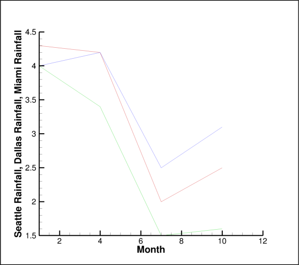
Attributes

`i_range`	`IndexRange` for the I dimension of ordered data.
`j_range`	`IndexRange` for the J dimension of ordered data.
`k_range`	`IndexRange` for the K dimension of ordered data.
`varying_index`	Family of lines to be drawn.

LinemapIndices.i_range¶

IndexRange for the I dimension of ordered data.

This example shows I-lines at i = [0, 2, 4, 6, 8, 10]:

>>> plot.linemap(0).indices.i_range = 0, 10, 2

Type:: tuple of integers (min, max, step)

LinemapIndices.j_range¶

IndexRange for the J dimension of ordered data.

This example shows all J-lines starting with j = 10 up to the maximum J-line of the associated Zone:

>>> plot.linemap(0).indices.j_range = 10, None, 1

Type:: tuple of integers (min, max, step)

LinemapIndices.k_range¶

IndexRange for the K dimension of ordered data.

This example shows all K-lines starting with the first up to 5 from the last K-line of the associated Zone:

>>> plot.linemap(0).indices.k_range = None, -5

Type:: tuple of integers (min, max, step)

LinemapIndices.varying_index¶

Family of lines to be drawn.

This is the order which varies along the lines drawn. K-varying is only available if the mapping is using an IJK-ordered zone:

>>> from tecplot.constant import IJKLines
>>> plot.linemap(0).indices.varying_index = IJKLines.J

Type:: IJKLines

LinemapSymbols ¶

class tecplot.plot.LinemapSymbols(linemap)[source]¶

Style control for markers placed along lines.

This class allows the user to set the style of the symbols to be shown including setting a geometric shape, text character, line and fill colors and spacing. The plot-level show_symbols attribute must be enabled to show symbols in any specific linemap within the plot:

from os import path
import tecplot as tp
from tecplot.constant import PlotType, Color, FillMode, GeomShape

examples_dir = tp.session.tecplot_examples_directory()
infile = path.join(examples_dir, 'SimpleData', 'Rainfall.dat')
dataset = tp.data.load_tecplot(infile)

frame = tp.active_frame()
frame.plot_type = PlotType.XYLine
plot = frame.plot()
plot.show_symbols = True

lmaps = plot.linemaps(0, 1, 2)

lmaps.symbols.show = True
lmaps.symbols.symbol().shape = GeomShape.Square
lmaps.symbols.size = 2.5
lmaps.symbols.color = Color.Blue
lmaps.symbols.line_thickness = 0.4
lmaps.symbols.fill_mode = FillMode.UseSpecificColor
lmaps.symbols.fill_color = Color.Azure

# save image to file
tp.export.save_png('linemap_symbols.png', 600, supersample=3)

Attributes

`color`	Edge or text `Color` of the drawn symbols.
`fill_color`	The fill or background color.
`fill_mode`	The fill mode for the background.
`line_thickness`	Width of the lines when drawing geometry symbols.
`show`	Display symbols along the lines to be drawn.
`size`	Size of the symbols to draw.
`step`	Space between symbols to be shown.
`step_mode`	Space the symbols by index or frame height.
`symbol_type`	The `SymbolType` to use for this linemap.

Methods

symbol([symbol_type])

Returns a linemap symbol style object.

LinemapSymbols.color¶

Edge or text Color of the drawn symbols.

Example usage:

>>> from tecplot.constant import Color
>>> plot.linemap(1).symbols.color = Color.Blue

Type:: Color

LinemapSymbols.fill_color¶

The fill or background color.

The fill_mode attribute must be set to FillMode.UseSpecificColor:

>>> from tecplot.constant import Color, FillMode
>>> symbols = plot.linemap(0).symbols
>>> symbols.fill_mode = FillMode.UseSpecificColor
>>> symbols.fill_color = Color.Yellow

Type:: Color

LinemapSymbols.fill_mode¶

The fill mode for the background.

Possible values: FillMode.UseSpecificColor, FillMode.UseLineColor,: FillMode.UseBackgroundColor or FillMode.None_.

Example usage:

>>> from tecplot.constant import Color, FillMode
>>> symbols = plot.linemap(0).symbols
>>> symbols.fill_mode = FillMode.UseBackgroundColor

Type:: FillMode

LinemapSymbols.line_thickness¶

Width of the lines when drawing geometry symbols.

Example usage:

>>> from tecplot.constant import SymbolType
>>> symbols = plot.linemap(0).symbols
>>> symbols.symbol_type = SymbolType.Geometry
>>> symbols.line_thickness = 0.8

Type:: float

LinemapSymbols.show¶

Display symbols along the lines to be drawn.

The parent plot object must have symbols enabled as well:

>>> plot.show_symbols = True
>>> plot.linemap(0).symbols.show = True

Type:: bool

LinemapSymbols.size¶

Size of the symbols to draw.

Example usage:

>>> plot.linemap(0).symbols.size = 3.5

Type:: float

LinemapSymbols.step¶

Space between symbols to be shown.

The step is specified either as a percentage of the frame height or as a number of indices to skip depending on the value of LinemapSymbols.step_mode. This example will add symbols to every third point:

>>> plot.linemap(0).symbols.step = 3

Type:: float

LinemapSymbols.step_mode¶

Space the symbols by index or frame height.

This example will make sure all symbols are no closer than 10% of the frame height to each other:

>>> from tecplot.constant import StepMode
>>> sym = plot.linemap(0).symbols
>>> sym.step_mode = StepMode.ByFrameUnits
>>> sym.step = 10

Type:: StepMode

LinemapSymbols.symbol(symbol_type=None)[source]¶

Returns a linemap symbol style object.

Parameters:: symbol_type (SymbolType, optional) – The type of symbol to return. By default, this will return the active symbol type which is obtained from LinemapSymbols.symbol_type.

Returns: TextSymbol or GeometrySymbol

Example usage:

>>> from tecplot.constant import SymbolType
>>> plot.linemap(0).symbols.symbol_type = SymbolType.Text
>>> symbol = plot.linemap(0).symbols.symbol()
>>> symbol.text = 'a'

LinemapSymbols.symbol_type¶

The SymbolType to use for this linemap.

Possible values are: SymbolType.Geometry, SymbolType.Text.

This sets the active symbol type. Use LinemapSymbols.symbol` to access the symbol:

>>> from tecplot.constant import SymbolType
>>> linemap = plot.linemap(0)
>>> linemap.symbols.symbol_type = SymbolType.Text
>>> symbol = linemap.symbols.symbol(SymbolType.Text)
>>> symbol.text = 'a'

Type:: SymbolType

GeometrySymbol ¶

class tecplot.plot.GeometrySymbol(parent, svarg='SYMBOLSHAPE')[source]¶

Geometric shape for linemap symbols.

from os import path
import tecplot as tp
from tecplot.constant import (PlotType, Color, GeomShape, SymbolType,
                              FillMode)

examples_dir = tp.session.tecplot_examples_directory()
infile = path.join(examples_dir, 'SimpleData', 'Rainfall.dat')
dataset = tp.data.load_tecplot(infile)

frame = tp.active_frame()
frame.plot_type = PlotType.XYLine
plot = frame.plot()
plot.show_symbols = True

cols = [Color.DeepRed, Color.Blue, Color.Fern]
shapes = [GeomShape.Square, GeomShape.Circle, GeomShape.Del]

lmaps = plot.linemaps()

lmaps.show = True
lmaps.symbols.show = True
lmaps.symbols.size = 4.5
lmaps.symbols.fill_mode = FillMode.UseSpecificColor
lmaps.symbols.symbol_type = SymbolType.Geometry

for lmap, color, shape in zip(lmaps, cols, shapes):
    lmap.line.color = color
    lmap.symbols.color = color
    lmap.symbols.fill_color = color
    lmap.symbols.symbol().shape = shape

plot.view.fit()

# save image to file
tp.export.save_png('linemap_symbols_geometry.png', 600, supersample=3)

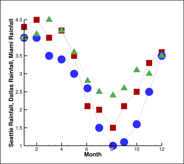
Attributes

shape

Geometric shape to use when plotting linemap symbols.

GeometrySymbol.shape¶

Geometric shape to use when plotting linemap symbols.

Possible values: Square, Del, Grad, RTri, LTri, Diamond, Circle, Cube, Sphere, Octahedron, Point.

Example usage:

>>> from tecplot.constant import SymbolType, GeomShape
>>> symbols = plot.linemap(0).symbols
>>> symbols.symbol_type = SymbolType.Geometry
>>> symbols.symbol().shape = GeomShape.Diamond

Type:: GeomShape

TextSymbol ¶

class tecplot.plot.TextSymbol(parent, svarg='SYMBOLSHAPE')[source]¶

Text character for linemap symbols.

Only a single character can be used.

from os import path
import tecplot as tp
from tecplot.constant import PlotType, Color, SymbolType, FillMode

examples_dir = tp.session.tecplot_examples_directory()
infile = path.join(examples_dir, 'SimpleData', 'Rainfall.dat')
dataset = tp.data.load_tecplot(infile)

frame = tp.active_frame()
frame.plot_type = PlotType.XYLine
plot = frame.plot()
plot.show_symbols = True

cols = [Color.DeepRed, Color.Blue, Color.Fern]
chars = ['S','D','M']

lmaps = plot.linemaps()
lmaps.show = True
lmaps.symbols.show = True
lmaps.symbols.size = 2.5
lmaps.symbols.color = Color.White
lmaps.symbols.fill_mode = FillMode.UseSpecificColor
lmaps.symbols.symbol_type = SymbolType.Text

for lmap, color, character in zip(lmaps, cols, chars):
    lmap.line.color = color
    lmap.symbols.fill_color = color
    lmap.symbols.symbol().text = character

plot.view.fit()

# save image to file
tp.export.save_png('linemap_symbols_text.png', 600, supersample=3)

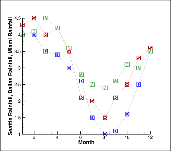
Attributes

`font_override`	Typeface to use when rendering text-based symbols.
`text`	The ASCII character to use as the symbol to show
`use_base_font`	Use the base typeface when rendering text-based symbols.

TextSymbol.font_override¶

Typeface to use when rendering text-based symbols.

Possible values: constant.Font.Greek, constant.Font.Math or constant.Font.UserDefined.

The use_base_font attribute must be set to False:

>>> from tecplot.constant import SymbolType, Font
>>> symbols = plot.linemap(0).symbols
>>> symbols.symbol_type = SymbolType.Text
>>> symbols.symbol().use_base_font = False
>>> symbols.symbol().font_override = Font.Greek

Type:: constant.Font

TextSymbol.text¶

The ASCII character to use as the symbol to show

Note

This is limited to a single character.

Example usage:

>>> from tecplot.constant import SymbolType
>>> symbols = plot.linemap(0).symbols
>>> symbols.symbol_type = SymbolType.Text
>>> symbols.symbol().text = 'X'

TextSymbol.use_base_font¶

Use the base typeface when rendering text-based symbols.

When False, the font_override attribute takes effect:

>>> from tecplot.constant import SymbolType, Font
>>> symbols = plot.linemap(0).symbols
>>> symbols.symbol_type = SymbolType.Text
>>> symbols.symbol().use_base_font = False
>>> symbols.symbol().font_override = Font.Greek

Type:: bool

Plot¶

Plots ¶

Cartesian2DFieldPlot ¶

Cartesian3DFieldPlot ¶

PolarLinePlot ¶

XYLinePlot ¶

SketchPlot ¶

Fieldmaps ¶

Cartesian2DFieldmap ¶

Cartesian2DFieldmapCollection ¶

Cartesian3DFieldmap ¶

Cartesian3DFieldmapCollection ¶

FieldmapContour ¶

FieldmapEdge ¶

FieldmapEffects ¶

FieldmapEffects3D ¶

FieldmapMesh ¶

FieldmapPoints ¶

FieldmapScatter ¶

GeometryScatterSymbol ¶

TextScatterSymbol ¶

FieldmapShade ¶

FieldmapShade3D ¶

FieldmapSurfaces ¶

FieldmapVector ¶

Linemaps ¶

PolarLinemap ¶

PolarLinemapCollection ¶

XYLinemap ¶

XYLinemapCollection ¶

LinemapLine ¶

LinemapCurve ¶

LinemapBars ¶

LinemapErrorBars ¶

LinemapIndices ¶

LinemapSymbols ¶

GeometrySymbol ¶

TextSymbol ¶

Table of Contents

This Page