Examples

Hello World

A simple “Hello, World!” adds text to the active frame and exports the frame to an image file.

import logging
logging.basicConfig(level=logging.DEBUG)

import tecplot

# Run this script with "-c" to connect to Tecplot 360 on port 7600
# To enable connections in Tecplot 360, click on:
#   "Scripting" -> "PyTecplot Connections..." -> "Accept connections"
import sys
if '-c' in sys.argv:
    tecplot.session.connect()

tecplot.new_layout()

frame = tecplot.active_frame()
frame.add_text('Hello, World!', position=(36, 50), size=34)
tecplot.export.save_png('hello_world.png', 600, supersample=3)

Loading Layouts

Layouts can be loaded with the tecplot.load_layout() method. This will accept both lay and lpk (packaged) files. The exported image interprets the image type by the extension you give it. See tecplot.export.save_png() for more details. Notice in this example, we turn on logging down to the DEBUG level which is extremely verbose. This is useful for debugging the connection between the script and Tecplot 360.

import logging
import os
import sys

logging.basicConfig(stream=sys.stdout, level=logging.INFO)

import tecplot

# Run this script with "-c" to connect to Tecplot 360 on port 7600
# To enable connections in Tecplot 360, click on:
#   "Scripting" -> "PyTecplot Connections..." -> "Accept connections"
import sys
if '-c' in sys.argv:
    tecplot.session.connect()

examples_dir = tecplot.session.tecplot_examples_directory()
infile = os.path.join(examples_dir, 'SimpleData', 'DuctFlow.lay')

tecplot.load_layout(infile)

# set some style to modify the plot
plot = tecplot.active_frame().plot()
plot.slices(0).edge.show = False

tecplot.export.save_png('layout_example.png', 600, supersample=3)

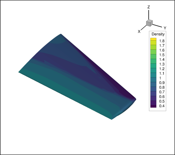
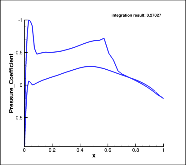
Extracting Slices

This script produces two images: a 3D view of the wing and a simplified pressure coefficient plot half-way down the wing:

import os
import sys
import logging

logging.basicConfig(stream=sys.stdout, level=logging.INFO)

import tecplot

# Run this script with "-c" to connect to Tecplot 360 on port 7600
# To enable connections in Tecplot 360, click on:
#   "Scripting" -> "PyTecplot Connections..." -> "Accept connections"
import sys
if '-c' in sys.argv:
    tecplot.session.connect()


examples_dir = tecplot.session.tecplot_examples_directory()
datafile = os.path.join(examples_dir, 'OneraM6wing', 'OneraM6_SU2_RANS.plt')
dataset = tecplot.data.load_tecplot(datafile)

frame = tecplot.active_frame()
frame.plot_type = tecplot.constant.PlotType.Cartesian3D
frame.plot().show_contour = True

# ensure consistent output between interactive (connected) and batch
frame.plot().contour(0).levels.reset_to_nice()

# export image of wing
tecplot.export.save_png('wing.png', 600, supersample=3)

# extract an arbitrary slice from the surface data on the wing
extracted_slice = tecplot.data.extract.extract_slice(
    origin=(0, 0.25, 0),
    normal=(0, 1, 0),
    source=tecplot.constant.SliceSource.SurfaceZones,
    dataset=dataset)

extracted_slice.name = 'Quarter-chord C_p'

# get x from slice
extracted_x = extracted_slice.values('x')

# copy of data as a numpy array
x = extracted_x.as_numpy_array()

# normalize x
xc = (x - x.min()) / (x.max() - x.min())
extracted_x[:] = xc

# switch plot type in current frame
frame.plot_type = tecplot.constant.PlotType.XYLine
plot = frame.plot()

# clear plot
plot.delete_linemaps()

# create line plot from extracted zone data
cp_linemap = plot.add_linemap(
    name=extracted_slice.name,
    zone=extracted_slice,
    x=dataset.variable('x'),
    y=dataset.variable('Pressure_Coefficient'))

# integrate over the normalized extracted slice values
# notice we have to convert zero-based index to one-based for CFDAnalyzer
tecplot.macro.execute_extended_command('CFDAnalyzer4', '''
    Integrate
    VariableOption='Average'
    XOrigin=0 YOrigin=0
    ScalarVar={scalar_var}
    XVariable=1
'''.format(scalar_var=dataset.variable('Pressure_Coefficient').index + 1))

# get integral result from Frame's aux data
total = float(frame.aux_data['CFDA.INTEGRATION_TOTAL'])

# overlay result on plot in upper right corner
frame.add_text('integration result: {:.5f}'.format(total), (60,90))

# set style of linemap plot
cp_linemap.line.color = tecplot.constant.Color.Blue
cp_linemap.line.line_thickness = 0.8
cp_linemap.y_axis.reverse = True

# update axes limits to show data
plot.view.fit()

# export image of pressure coefficient as a function of x/c
tecplot.export.save_png('wing_pressure_coefficient.png', 600, supersample=3)

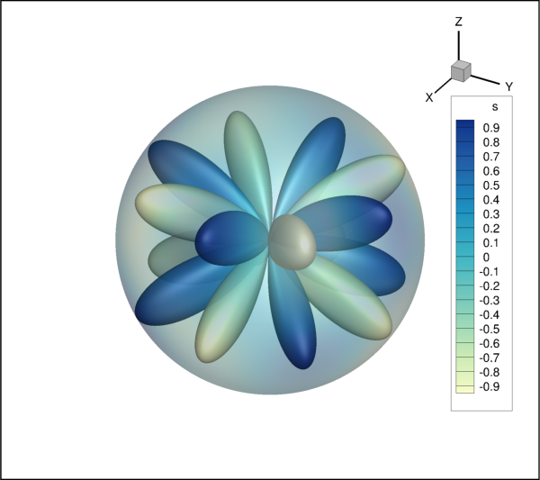
Numpy Integration

Note

Numpy, SciPy Required

This example requires both numpy and scipy installed. SciPy, in turn, requires a conforming linear algebra system such as OpenBLAS, LAPACK, ATLAS or MKL. It is recommended to use your operating system’s package manager to do this. Windows users and/or users that do not have root access to their machines might consider using Anaconda to setup a virtual environment where they can install python, numpy, scipy and all of its dependencies.

The spherical harmonic (n,m) = (5,4) is calculated at unit radius. The magnitude is then used to create a 3D shape. The plot-style is modified and the following image is exported.

import logging as log
import numpy as np
from numpy import abs, pi, cos, sin
from scipy import special

log.basicConfig(level=log.INFO)

import tecplot as tp
from tecplot.session import set_style
from tecplot.constant import ColorMapDistribution

# Run this script with "-c" to connect to Tecplot 360 on port 7600
# To enable connections in Tecplot 360, click on:
#   "Scripting" -> "PyTecplot Connections..." -> "Accept connections"
import sys
if '-c' in sys.argv:
    tp.session.connect()

shape = (200, 600)

log.info('creating spherical harmonic data')
r = 0.3
phi = np.linspace(0, pi, shape[0])
theta = np.linspace(0, 2*pi, shape[1])

ttheta, pphi = np.meshgrid(theta, phi, indexing='ij')

xx = r * sin(pphi) * cos(ttheta)
yy = r * sin(pphi) * sin(ttheta)
zz = r * cos(pphi)

n = 5
m = 4

ss = special.sph_harm(m, n, ttheta, pphi).real
ss /= ss.max()

'''
The tecplot.session.suspend() context can be used to improve the performance
of a series of operations including data creation and style setting. It
effectively prevents the Tecplot 360 interface from trying to "keep up" with
changes on the fly. In this short example, the difference in performance is
still small, but it serves to demonstrate how and when to use this context.
'''
with tp.session.suspend():
    log.info('creating tecplot dataset')
    ds = tp.active_frame().create_dataset('Data', ['x','y','z','s'])

    sphere_zone = ds.add_ordered_zone(
        'SphericalHarmonic({}, {}) Sphere'.format(m, n),
        shape)

    sphere_zone.values('x')[:] = xx.ravel()
    sphere_zone.values('y')[:] = yy.ravel()
    sphere_zone.values('z')[:] = zz.ravel()
    sphere_zone.values('s')[:] = ss.ravel()

    log.info('creating shaped zone')
    shaped_zone = ds.add_ordered_zone(
        'SphericalHarmonic({}, {}) Shaped'.format(m, n),
        shape)

    shaped_zone.values('x')[:] = (abs(ss)*xx).ravel()
    shaped_zone.values('y')[:] = (abs(ss)*yy).ravel()
    shaped_zone.values('z')[:] = (abs(ss)*zz).ravel()
    shaped_zone.values('s')[:] = ss.ravel()

    log.info('setting plot type to Cart3D')
    tp.active_frame().plot_type = tp.constant.PlotType.Cartesian3D

    plot = tp.active_frame().plot()

    '''
    The lines below are equivalent to the macro commands.

    Notice that PyTecplot indexes universally from zero where the
    macro indexes from one.

    $!FIELDLAYERS SHOWCONTOUR = YES
    $!FIELDLAYERS USETRANSLUCENCY = YES
    $!FIELDMAP [1]  EFFECTS { SURFACETRANSLUCENCY = 70 }
    $!FIELDMAP [2]  EFFECTS { SURFACETRANSLUCENCY = 30 }
    $!GLOBALCONTOUR 1  COLORMAPFILTER { COLORMAPDISTRIBUTION = CONTINUOUS }
    $!GLOBALCONTOUR 1  COLORMAPNAME = 'Sequential - Yellow/Green/Blue'
    '''
    plot.show_contour = True
    plot.use_translucency = True
    plot.fieldmap(sphere_zone).effects.surface_translucency = 70
    plot.fieldmap(shaped_zone).effects.surface_translucency = 30
    plot.contour(0).colormap_filter.distribution = ColorMapDistribution.Continuous
    plot.contour(0).colormap_name = 'Sequential - Yellow/Green/Blue'

    for axis in plot.axes:
        axis.fit_range()

    log.info('exiting suspend context')

log.info('continuing with script')

# ensure consistent output between interactive (connected) and batch
tp.active_frame().plot().contour(0).levels.reset_to_nice()

filename = 'spherical_harmonic_{}_{}'.format(m, n)

log.info('saving image')
tp.export.save_png(filename + '.png', 600, supersample=3)

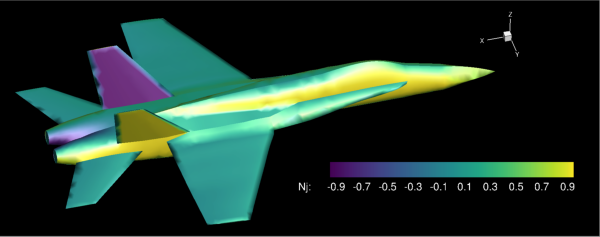
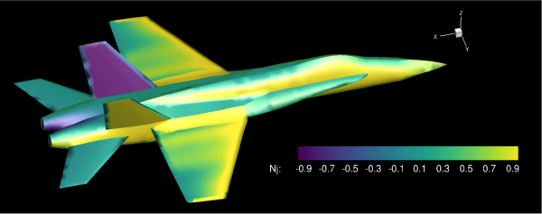
Execute Equation

This example illustrates altering data through equations in two zones. For complete information on the Tecplot Engine “data alter” syntax, see Chapter 21, Data Operations, in the Tecplot 360 User’s Manual. This script outputs the original data followed by the same image where we’ve modified the scaling of Nj only on the wings.

import os
import tecplot

# Run this script with "-c" to connect to Tecplot 360 on port 7600
# To enable connections in Tecplot 360, click on:
#   "Scripting" -> "PyTecplot Connections..." -> "Accept connections"
import sys
if '-c' in sys.argv:
    tecplot.session.connect()

examples_dir = tecplot.session.tecplot_examples_directory()
infile = os.path.join(examples_dir, 'SimpleData', 'F18.lay')

# Load a stylized layout where the contour variable is set to 'Nj'
tecplot.load_layout(infile)
current_dataset = tecplot.active_frame().dataset

# export original image
tecplot.export.save_png('F18_orig.png', 600, supersample=3)

# alter variable 'Nj' for the the two wing zones in the dataset
# In this simple example, just multiply it by 10.
tecplot.data.operate.execute_equation('{Nj}={Nj}*10',
    zones=[current_dataset.zone('right wing'),
           current_dataset.zone('left wing')])

# The contour color of the wings in the exported image will now be
# red, since we have altered the 'Nj' variable by multiplying it by 10.
tecplot.export.save_png('F18_altered.png', 600, supersample=3)

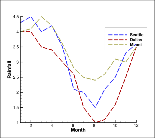
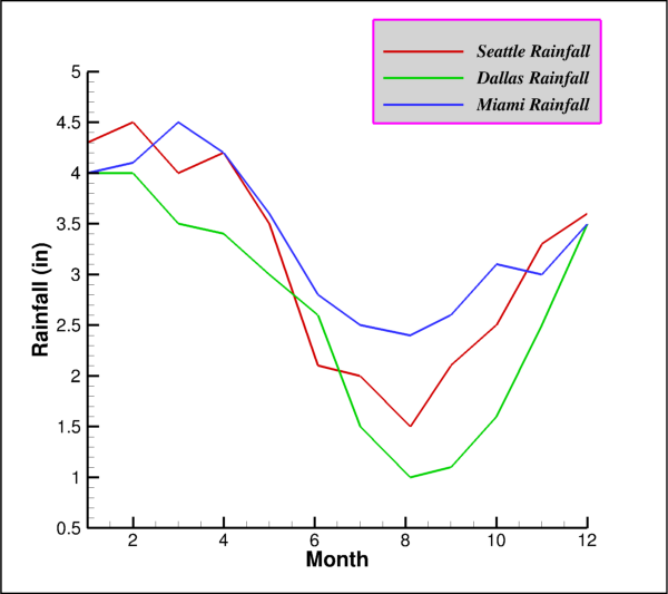
Line Plots

This example shows how to set the style for a plot of three lines. The y-axis label and legend labels are changed and the axes are adjusted to fit the data.

from os import path
import tecplot as tp
from tecplot.constant import PlotType, Color, LinePattern, AxisTitleMode

# Run this script with "-c" to connect to Tecplot 360 on port 7600
# To enable connections in Tecplot 360, click on:
#   "Scripting" -> "PyTecplot Connections..." -> "Accept connections"
import sys
if '-c' in sys.argv:
    tp.session.connect()

# load data from examples directory
examples_dir = tp.session.tecplot_examples_directory()
infile = path.join(examples_dir, 'SimpleData', 'Rainfall.dat')
dataset = tp.data.load_tecplot(infile)

# get handle to the active frame and set plot type to XY Line
frame = tp.active_frame()
frame.plot_type = PlotType.XYLine
plot = frame.plot()

# We will set the name, color and a few other properties
# for the first three linemaps in the dataset.
names = ['Seattle', 'Dallas', 'Miami']
colors = [Color.Blue, Color.DeepRed, Color.Khaki]

# loop over the linemaps, setting style for each
for lmap,name,color in zip(plot.linemaps(),names,colors):
    lmap.show = True
    lmap.name = name # This will be used in the legend

    # Changing some line attributes
    line = lmap.line
    line.color = color
    line.line_thickness = 1
    line.line_pattern = LinePattern.LongDash
    line.pattern_length = 2

# Set the y-axis label
plot.axes.y_axis(0).title.title_mode = AxisTitleMode.UseText
plot.axes.y_axis(0).title.text = 'Rainfall'

# Turn on legend
plot.legend.show = True

# Adjust the axes limits to show all the data
plot.view.fit()

# save image to file
tp.export.save_png('linemap.png', 600, supersample=3)

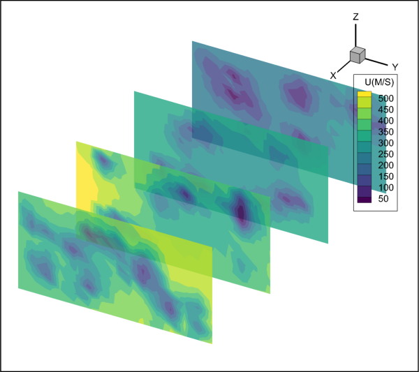
Creating Slices

This example illustrates reading a dataset then creating and showing arbitrary slices of the dataset. A primary slice, start, end, and 2 intermediate slices are shown.

from os import path
import tecplot as tp
from tecplot.constant import SliceSurface, ContourType

# Run this script with "-c" to connect to Tecplot 360 on port 7600
# To enable connections in Tecplot 360, click on:
#   "Scripting" -> "PyTecplot Connections..." -> "Accept connections"
import sys
if '-c' in sys.argv:
    tp.session.connect()

examples_dir = tp.session.tecplot_examples_directory()
datafile = path.join(examples_dir, 'SimpleData', 'DuctFlow.plt')
dataset = tp.data.load_tecplot(datafile)

plot = tp.active_frame().plot()
plot.contour(0).variable = dataset.variable('U(M/S)')
plot.show_contour = True

# Turn on slice and get handle to slice object
plot.show_slices = True
slice_0 = plot.slice(0)

# Turn on slice translucency
slice_0.effects.use_translucency = True
slice_0.effects.surface_translucency = 20

# Setup 4 evenly spaced slices
slice_0.show_primary_slice = False
slice_0.show_start_and_end_slices = True
slice_0.show_intermediate_slices = True
slice_0.start_position = (-.21, .05, .025)
slice_0.end_position = (1.342, .95, .475)
slice_0.num_intermediate_slices = 2

# Turn on contours of X Velocity on the slice
slice_0.contour.show = True
plot.contour(0).levels.reset_to_nice()

tp.export.save_png('slices.png', 600, supersample=3)

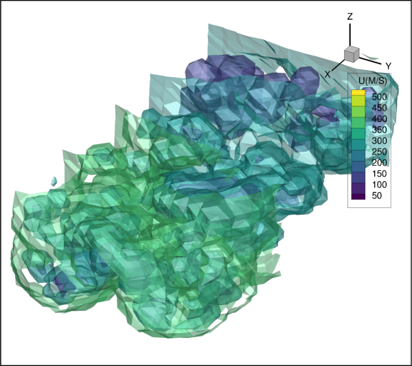
Creating Iso-surfaces

This example illustrates reading a dataset, then creating and showing isosurfaces.

from os import path

import tecplot as tp
from tecplot.constant import LightingEffect, IsoSurfaceSelection

# Run this script with "-c" to connect to Tecplot 360 on port 7600
# To enable connections in Tecplot 360, click on:
#   "Scripting" -> "PyTecplot Connections..." -> "Accept connections"
import sys
if '-c' in sys.argv:
    tp.session.connect()

examples_dir = tp.session.tecplot_examples_directory()
datafile = path.join(examples_dir, 'SimpleData', 'DuctFlow.plt')
dataset = tp.data.load_tecplot(datafile)

plot = tp.active_frame().plot()
plot.contour(0).variable = dataset.variable('U(M/S)')

plot.show_isosurfaces = True

iso = plot.isosurface(0)

iso.isosurface_selection = IsoSurfaceSelection.ThreeSpecificValues
iso.isosurface_values = (135.674706817, 264.930212259, 394.185717702)

iso.shade.use_lighting_effect = True
iso.effects.lighting_effect = LightingEffect.Paneled
iso.contour.show = True
iso.effects.use_translucency = True
iso.effects.surface_translucency = 50

# ensure consistent output between interactive (connected) and batch
plot.contour(0).levels.reset_to_nice()

tp.export.save_png('isosurface_example.png', 600, supersample=3)

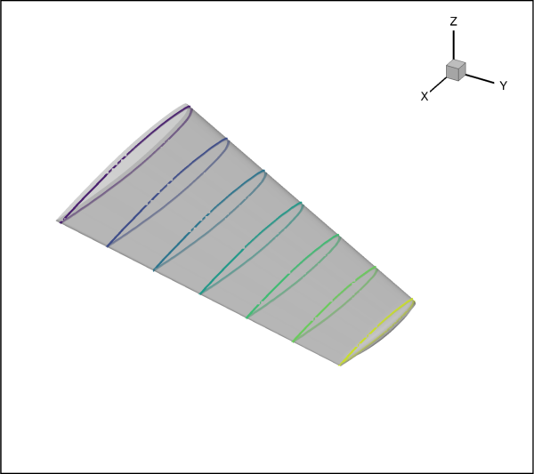
Wing Surface Slices

This example illustrates reading a dataset and showing surface slices with colored mesh on the Onera M6 Wing. Seven surface slices are shown, colored by the distance along the Y axis.

import tecplot
from tecplot.constant import *
import os
import numpy as np

# Run this script with "-c" to connect to Tecplot 360 on port 7600
# To enable connections in Tecplot 360, click on:
#   "Scripting" -> "PyTecplot Connections..." -> "Accept connections"
import sys
if '-c' in sys.argv:
    tecplot.session.connect()

examples_dir = tecplot.session.tecplot_examples_directory()
datafile = os.path.join(examples_dir, 'OneraM6wing', 'OneraM6_SU2_RANS.plt')
dataset = tecplot.data.load_tecplot(datafile)

frame = tecplot.active_frame()
plot = frame.plot()

# Setup First Contour Group to color by the distance along the Y axis (Span)
cont = plot.contour(0)
cont.variable = frame.dataset.variable('y')
cont.levels.reset_levels(np.linspace(0,1.2,13))
cont.legend.show = False

# Turn on only the periodic slices (start, end and intermeidate)
# and set them to span the length of the wing
plot.show_slices = True
slices = plot.slice(0)
slices.show = True
slices.slice_source = SliceSource.SurfaceZones
slices.orientation = SliceSurface.YPlanes
slices.show_primary_slice = False
slices.show_start_and_end_slices = True
slices.show_intermediate_slices = True
slices.num_intermediate_slices = 5
slices.start_position = (0, 0.02, 0)
slices.end_position = (0,1.19,0)

# Color the Surface Slices by the contour, this must be done on the mesh
slices.contour.show = False
slices.mesh.show = True
slices.mesh.color = cont
slices.mesh.line_thickness = 0.6
slices.edge.show = False

# Turn translucency on globally
plot.use_translucency = True

tecplot.export.save_png("wing_slices.png",600, supersample=3)

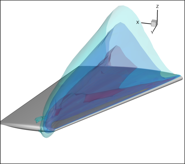
Mach Iso-surfaces

This example illustrates using contour group properties to define multiple Iso-surfaces. In this case, multiple Mach values are shown as Iso-surfaces.

import tecplot
from tecplot.constant import *
import os

# Run this script with "-c" to connect to Tecplot 360 on port 7600
# To enable connections in Tecplot 360, click on:
#   "Scripting" -> "PyTecplot Connections..." -> "Accept connections"
import sys
if '-c' in sys.argv:
    tecplot.session.connect()

examples_dir = tecplot.session.tecplot_examples_directory()
datafile = os.path.join(examples_dir, 'OneraM6wing', 'OneraM6_SU2_RANS.plt')
ds = tecplot.data.load_tecplot(datafile)

frame = tecplot.active_frame()
plot = frame.plot()

# Set Isosurface to match Contour Levels of the first group.
iso = plot.isosurface(0)
iso.isosurface_selection = IsoSurfaceSelection.AllContourLevels
cont = plot.contour(0)
iso.definition_contour_group = cont
cont.colormap_name = 'Magma'

# Setup definition Isosurface layers
cont.variable = ds.variable('Mach')
cont.levels.reset_levels( [.95,1.0,1.1,1.4])
print(list(cont.levels))

# Turn on Translucency
iso.effects.use_translucency = True
iso.effects.surface_translucency = 80

# Turn on Isosurfaces
plot.show_isosurfaces = True
iso.show = True

cont.legend.show = False

view = plot.view
view.psi = 65.777
view.theta = 166.415
view.alpha = -1.05394
view.position = (-23.92541680486183, 101.8931504712126, 47.04269529295333)
view.width = 1.3844

tecplot.export.save_png("wing_iso.png",width=600, supersample=3)

Exception Handling

It is the policy of the PyTecplot Python module to raise exceptions on any failure. It is the user’s job to catch them or otherwise prevent them by ensuring the Tecplot Engine is properly setup to the task you ask of it. Aside from exceptions raised by the underlying Python core libraries, PyTecplot may raise a subclass of TecplotError, the most common being TecplotRuntimeError.

import logging
import os

# turn on exceptionally verbose logging!!!
logging.basicConfig(level=logging.DEBUG)

import tecplot
from tecplot.exception import *

'''
Calling tecplot.session.acquire_license() is optional.
If you do not call it, it will be called automatically for you
the first time you call any PyTecplot API.

acquire_license() may also be called manually. It will raise an exception
if Tecplot cannot be initialized. The most common reason that
Tecplot cannot be initialized is if a valid license is not found.
If you call start yourself, you can catch and recover from the
exception.

Note that calling tecplot.session.stop() will release the license acquired
when calling tecplot.session.connect().

Also note that once tecplot.session.stop() is called, the Tecplot Engine
cannot be restarted again during the current python session.
'''
try:
    tecplot.session.acquire_license()
except TecplotLicenseError:
    logging.exception('Missing or invalid license:')
except TecplotLogicError:
    # It is a logic error when acquiring license when
    # already connected to Tecplot 360 TecUtil Server
    if not tecplot.session.connected():
        raise
except TecplotError:
    logging.exception('Could not initialize pytecplot')
    exit(1)

examples_dir = tecplot.session.tecplot_examples_directory()
infile = os.path.join(examples_dir, 'SimpleData', 'SpaceShip.lpk')
outfile = 'spaceship.png'

try:
    logging.info('Opening layout file: ' + infile)
    tecplot.load_layout(infile)

    logging.info('Exporting Image: ' + outfile)
    tecplot.export.save_png(outfile, 600, supersample=3)

    logging.info('Finished, no errors')

except IOError:
    logging.debug("I/O Error: Check disk space and permissions")
except TecplotSystemError:
    logging.exception('Failed to export image: ' + outfile)
finally:
    # tecplot.session.stop() may be called manually to
    # shut down Tecplot and release the license.
    # If tecplot.session.stop() is not called manually
    # it will be called automatically when the script exits.
    tecplot.session.stop()

logging.info('Done')

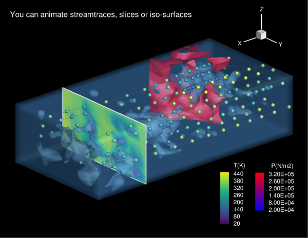
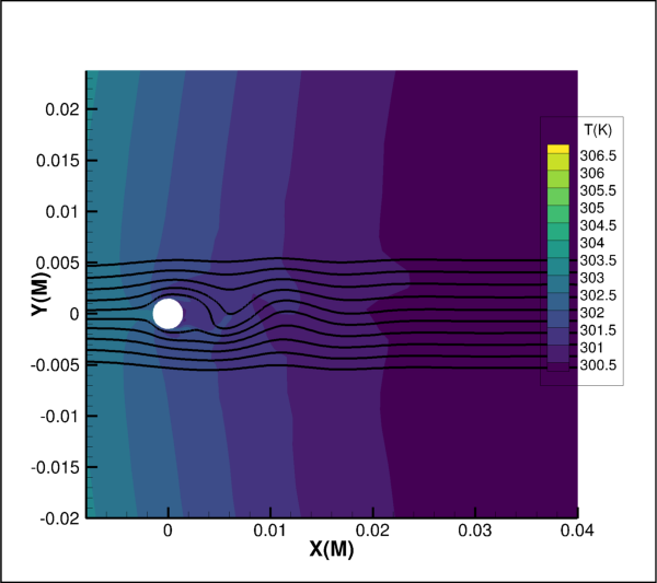
Streamtraces

Using the transient Vortex Shedding layout a rake of 2D streamtrace lines are added.

import tecplot
from tecplot.constant import *
import os

# Run this script with "-c" to connect to Tecplot 360 on port 7600
# To enable connections in Tecplot 360, click on:
#   "Scripting" -> "PyTecplot Connections..." -> "Accept connections"
import sys
if '-c' in sys.argv:
    tecplot.session.connect()

examples_dir = tecplot.session.tecplot_examples_directory()
datafile = os.path.join(examples_dir, 'SimpleData', 'VortexShedding.plt')
dataset = tecplot.data.load_tecplot(datafile)

frame = tecplot.active_frame()
frame.plot_type = tecplot.constant.PlotType.Cartesian2D

# Setup up vectors and background contour
plot = frame.plot()
plot.vector.u_variable = dataset.variable('U(M/S)')
plot.vector.v_variable = dataset.variable('V(M/S)')
plot.contour(0).variable = dataset.variable('T(K)')
plot.show_streamtraces = True
plot.show_contour = True
plot.fieldmap(0).contour.show = True

# Add streamtraces and set streamtrace style
streamtraces = plot.streamtraces
streamtraces.add_rake(start_position=(-0.003, 0.005),
                      end_position=(-0.003, -0.005),
                      stream_type=Streamtrace.TwoDLine,
                      num_seed_points=10)

streamtraces.show_arrows = False
streamtraces.line_thickness = .4

plot.axes.y_axis.min = -0.02
plot.axes.y_axis.max = 0.02
plot.axes.x_axis.min = -0.008
plot.axes.x_axis.max = 0.04

tecplot.export.save_png('streamtrace_2D.png', 600, supersample=3)

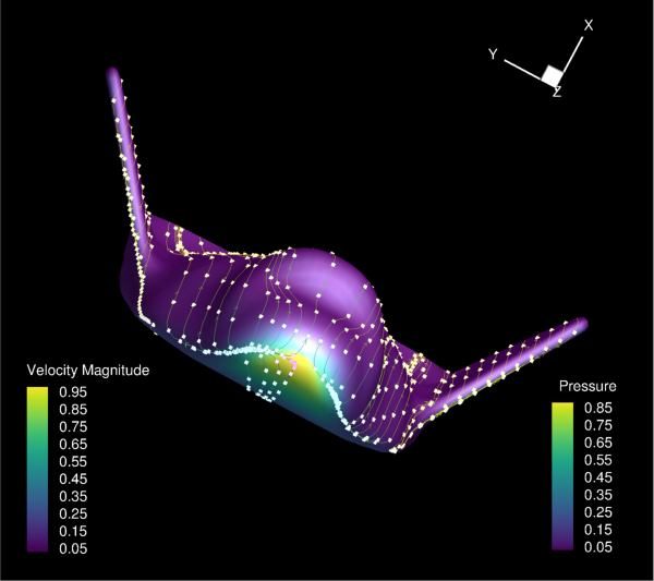
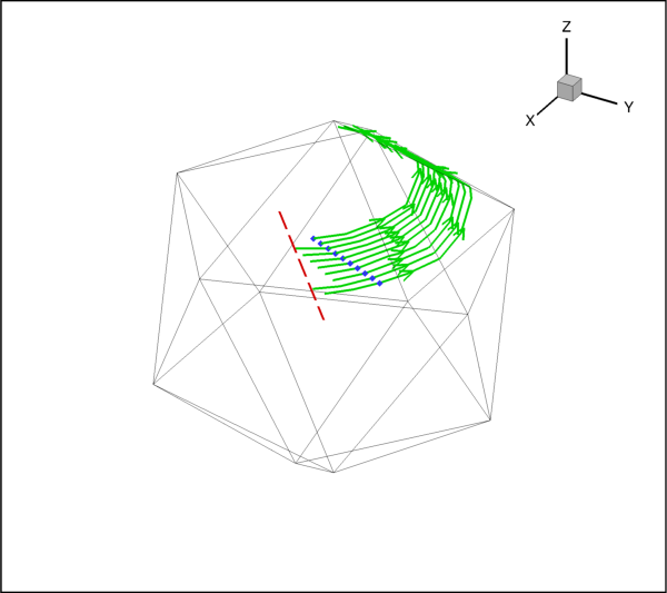
This example illustrates adding a rake of streamtraces.

import os
import tecplot
from tecplot.constant import *
from tecplot.plot import Cartesian3DFieldPlot

# Run this script with "-c" to connect to Tecplot 360 on port 7600
# To enable connections in Tecplot 360, click on:
#   "Scripting" -> "PyTecplot Connections..." -> "Accept connections"
import sys
if '-c' in sys.argv:
    tecplot.session.connect()

examples_dir = tecplot.session.tecplot_examples_directory()
datafile = os.path.join(examples_dir, 'SimpleData', 'Eddy.plt')
dataset = tecplot.data.load_tecplot(datafile)

frame = tecplot.active_frame()
frame.plot_type = tecplot.constant.PlotType.Cartesian3D

plot = frame.plot()
plot.fieldmap(0).surfaces.surfaces_to_plot = SurfacesToPlot.BoundaryFaces
plot.show_mesh = True
plot.show_shade = False

plot.vector.u_variable_index = 4
plot.vector.v_variable_index = 5
plot.vector.w_variable_index = 6
plot.show_streamtraces = True

streamtrace = plot.streamtraces
streamtrace.color = Color.Green

streamtrace.show_paths = True
streamtrace.show_arrows = True
streamtrace.arrowhead_size = 3
streamtrace.step_size = .25
streamtrace.line_thickness = .4
streamtrace.max_steps = 10

# Streamtraces termination line:
streamtrace.set_termination_line([(-25.521, 39.866),
                                  (-4.618, -11.180)])

# Streamtraces will stop at the termination line when active
streamtrace.termination_line.active = True

# We can also show the termination line itself
streamtrace.termination_line.show = True
streamtrace.termination_line.color = Color.Red
streamtrace.termination_line.line_thickness = 0.4
streamtrace.termination_line.line_pattern = LinePattern.LongDash

# Markers
streamtrace.show_markers = True
streamtrace.marker_color = Color.Blue
streamtrace.marker_symbol_type = SymbolType.Geometry
streamtrace.marker_symbol().shape = GeomShape.Diamond

# Add surface line streamtraces
streamtrace.add_rake(start_position=(45.49, 15.32, 59.1),
                     end_position=(48.89, 53.2, 47.6),
                     stream_type=Streamtrace.SurfaceLine)


tecplot.export.save_png('streamtrace_line_example.png', 600, supersample=3)

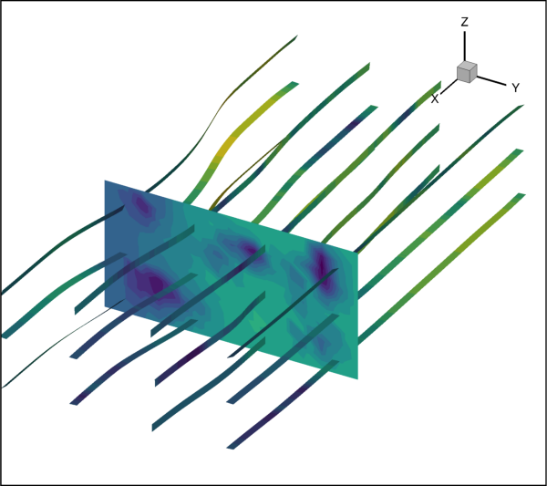
This example illustrates adding ribbon streamtrace.

import os
import tecplot
from tecplot.constant import *
import numpy as np

# Run this script with "-c" to connect to Tecplot 360 on port 7600
# To enable connections in Tecplot 360, click on:
#   "Scripting" -> "PyTecplot Connections..." -> "Accept connections"
import sys
if '-c' in sys.argv:
    tecplot.session.connect()

examples_dir = tecplot.session.tecplot_examples_directory()
datafile = os.path.join(examples_dir, 'SimpleData', 'DuctFlow.plt')
dataset = tecplot.data.load_tecplot(datafile)

frame = tecplot.active_frame()
frame.plot_type = tecplot.constant.PlotType.Cartesian3D

plot = frame.plot()
plot.contour(0).variable = dataset.variable('P(N/m2)')
plot.contour(0).levels.reset_to_nice()
plot.contour(0).legend.show = False

plot.vector.u_variable = dataset.variable('U(M/S)')
plot.vector.v_variable = dataset.variable('V(M/S)')
plot.vector.w_variable = dataset.variable('W(M/S)')

# Goal: create a grid of 12 stream trace ribbons on a slice
x_slice_location = .79
y_start = .077
y_end = .914
z_start = .052
z_end = .415

num_left_right_slices = 4  # Must be >= 2
num_top_bottom_slices = 3  # Must be >= 2


# Show and add a slice.
plot.show_slices = True
slice_0 = plot.slice(0)

# Set the x position of the slice.
slice_0.origin = [x_slice_location, 0, 0]

slice_0.contour.show = True

plot.show_streamtraces = True
streamtraces = plot.streamtraces
streamtraces.show_paths = True

rod = streamtraces.rod_ribbon
rod.width = .03
rod.contour.show = True


for y in np.linspace(y_start, y_end, num=num_left_right_slices):
    for z in np.linspace(z_start, z_end, num=num_top_bottom_slices):
        streamtraces.add([x_slice_location,y,z], Streamtrace.VolumeRibbon)

tecplot.export.save_png('streamtrace_ribbon_example.png', 600, supersample=3)

Line Legend

This example illustrates displaying an XY line legend and changing its attributes.

import os

import tecplot
from tecplot.constant import *

# Run this script with "-c" to connect to Tecplot 360 on port 7600
# To enable connections in Tecplot 360, click on:
#   "Scripting" -> "PyTecplot Connections..." -> "Accept connections"
import sys
if '-c' in sys.argv:
    tecplot.session.connect()

examples_dir = tecplot.session.tecplot_examples_directory()
datafile = os.path.join(examples_dir, 'SimpleData', 'Rainfall.dat')
dataset = tecplot.data.load_tecplot(datafile)

frame = tecplot.active_frame()
plot = frame.plot()
frame.plot_type = tecplot.constant.PlotType.XYLine

for i in range(3):
    plot.linemap(i).show = True
    plot.linemap(i).line.line_thickness = .4

y_axis = plot.axes.y_axis(0)
y_axis.title.title_mode = AxisTitleMode.UseText
y_axis.title.text = 'Rainfall (in)'
y_axis.fit_range_to_nice()

legend = plot.legend
legend.show = True
legend.box.box_type = TextBox.Filled
legend.box.color = Color.Purple
legend.box.fill_color = Color.LightGrey
legend.box.line_thickness = .4
legend.box.margin = 5

legend.anchor_alignment = AnchorAlignment.MiddleRight
legend.row_spacing = 1.5
legend.show_text = True
legend.font.typeface = 'Arial'
legend.font.italic = True

legend.text_color = Color.Black
legend.position = (90, 88)

tecplot.export.save_png('legend_line.png', 600, supersample=3)

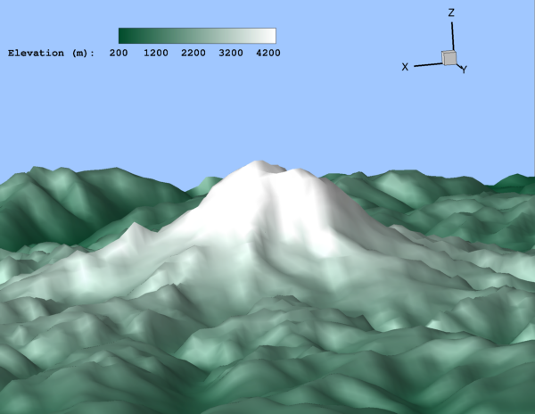
Contour Legend

This example illustrates displaying a contour legend and changing its attributes.

import os

import numpy as np

import tecplot
from tecplot.constant import *

# Run this script with "-c" to connect to Tecplot 360 on port 7600
# To enable connections in Tecplot 360, click on:
#   "Scripting" -> "PyTecplot Connections..." -> "Accept connections"
import sys
if '-c' in sys.argv:
    tecplot.session.connect()

# By loading a layout many style and view properties are set up already
examples_dir = tecplot.session.tecplot_examples_directory()
datafile = os.path.join(examples_dir, 'SimpleData', 'RainierElevation.lay')
tecplot.load_layout(datafile)

frame = tecplot.active_frame()
plot = frame.plot()

# Rename the elevation variable
frame.dataset.variable('E').name = "Elevation (m)"

# Set the levels to nice values
plot.contour(0).levels.reset_levels(np.linspace(200,4400,22))

legend = plot.contour(0).legend
legend.show = True
legend.vertical = False  # Horizontal
legend.auto_resize = False
legend.label_step = 5

legend.overlay_bar_grid = False
legend.position = (55, 94)  # Frame percentages

legend.box.box_type = TextBox.None_ # Remove Text box

legend.header.font.typeface = 'Courier'
legend.header.font.bold = True

legend.number_font.typeface = 'Courier'
legend.number_font.bold = True

tecplot.export.save_png('legend_contour.png', 600, supersample=3)

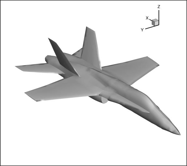
3D View

This example illustrates changing the attributes of the 3D view.

import tecplot
import os
from tecplot.constant import *

# Run this script with "-c" to connect to Tecplot 360 on port 7600
# To enable connections in Tecplot 360, click on:
#   "Scripting" -> "PyTecplot Connections..." -> "Accept connections"
import sys
if '-c' in sys.argv:
    tecplot.session.connect()

examples_dir = tecplot.session.tecplot_examples_directory()
infile = os.path.join(examples_dir, 'SimpleData', 'F18.plt')
ds = tecplot.data.load_tecplot(infile)
plot = tecplot.active_frame().plot(PlotType.Cartesian3D)
plot.activate()
plot.view.width = 17.5
plot.view.alpha = 0
plot.view.theta = 125
plot.view.psi = 65
plot.view.position = (-100, 80, 65)

tecplot.export.save_png('3D_view.png', 600, supersample=3)

Embedding LaTeX

This example shows how to create a text annotation in LaTeX mode.

import tecplot as tp
from tecplot.constant import *

frame = tp.active_frame()
frame.add_latex(r'''$
    \rho\frac{D\vec{u}}{Dt} =
        -\vec{\nabla}p + \vec{\nabla}\cdot\vec{\tau} + \rho\vec{g}
    $''', (50,50), size=32, anchor=TextAnchor.Center)

tp.export.save_png('latex_annotation.png')

Multiprocessing

This example shows how to use PyTecplot with Python’s Multiprocessing module.

import atexit, os, multiprocessing, sys
import tecplot as tp


def init(datafile, stylesheet):
    # !!! IMPORTANT !!!
    # Must register stop at exit to ensure Tecplot cleans
    # up all temporary files and does not create a core dump
    atexit.register(tp.session.stop)

    # Load data and apply a style sheet - done only once for all workers
    tp.data.load_tecplot(datafile)
    tp.active_frame().load_stylesheet(stylesheet)


def work(solution_time):
    # set solution time and save off image
    tp.active_frame().plot().solution_time = solution_time
    tp.export.save_png('img{0:.8f}.png'.format(solution_time))


if __name__ == '__main__':
    if sys.version_info < (3, 5):
        raise Exception('This example requires Python version 3.5+')
    if tp.session.connected():
        raise Exception('This example must be run in batch mode')

    # !!! IMPORTANT !!!
    # On Linux systems, Python's multiprocessing start method
    # defaults to "fork" which is incompatible with PyTecplot
    # and must be set to "spawn"
    multiprocessing.set_start_method('spawn')

    # Get the datafile, stylesheet and job parameters (solution times)
    examples_dir = tp.session.tecplot_examples_directory()
    datafile = os.path.join(examples_dir, 'SimpleData', 'VortexShedding.plt')
    stylesheet = os.path.join(examples_dir, 'SimpleData', 'VortexShedding.sty')

    # for this example, we are only processing the first MAXJOBS solution times
    MAXJOBS = 4
    solution_times = list(tp.data.load_tecplot(datafile).solution_times)[:MAXJOBS]

    # Set up the pool with initializing function and associated arguments
    num_workers = min(multiprocessing.cpu_count(), len(solution_times))
    pool = multiprocessing.Pool(num_workers, initializer=init, initargs=(datafile, stylesheet))

    try:
        # Map the work function to each of the job arguments
        pool.map(work, solution_times)
    finally:
        # !!! IMPORTANT !!!
        # Must join the process pool before parent script exits
        # to ensure Tecplot cleans up all temporary files
        # and does not create a core dump
        pool.close()
        pool.join()