To view a 2D plot of a loaded grid file, choose “2D Grid” from the Plot Type menu. The plot will change and the 2D Grid Plot Controls sidebar will appear.
|
|
 You can un-dock the Plot Controls sidebar by dragging its title bar to a new position. To put the Plot Controls back on the side of the workspace, double-click on its title bar (the region that displays the words “Plot Controls”). Or you can drag its title bar to either side of the workspace and let go, and it will snap into place.
The sidebar for 2D Grid plots has the options described following.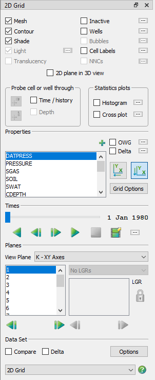
• Mesh Layer This toggle turns on or off the grid mesh.
• Contour Layer The Contour toggle controls display of the flooded contours, either as a solid color in each cell or bands of constant color.
• Connect When displaying wells, the Connect toggle turns on and off the lines connecting the well nodes.
• Shade Layer You can control the Shade only when Contour is toggled-off. Use this toggle to turn on or off the surface shading, making the interior of the grid mesh visible or hidden.
• Inactive Cells Toggle-on “Inactive” to display the inactive cells along with the active cells in your grid. If you have not loaded the inactive cells associated with the active grid, Tecplot RS will prompt you load them. See Section “Loading Inactive Cells” for details. See Section 14 - 1.6 “Inactive Cells” for information on how to display solution data on inactive cells.
• NNCs (2D Grid plots) Toggle-on this option to make Non-Neighbor Connections (NNCs) visible. Use the Details button to display the NNC dialog.
• Wells Toggle-on “Wells” to display any wells in the current plot. The shape of the symbol indicates the type of well (producer, injector, and so forth). The Details button adjacent to Wells brings up the Wells dialog.
• Bubble Plots Toggle-on “Bubbles” to show well data represented as bubbles on the well heads.
• Cell Labels Toggle-on “Cell Labels” to include cell or well labels in your plot.
• Time/History Toggling-on “Time/History” creates a new frame that you can use to display an XY line plot. You can choose to plot value versus time for a single cell in the grid or for a selected well. The current variables chosen in the XY Variables plot type determines the variables shown in the Time/History plots.
• Depth If you include RFT data in your current XY data set, you can plot them in a manner similar to the Time/History plots by toggling-on “Depth”. You can choose which variables to display by using the RFT Plots plot type.
• Statstics Displays or hides a statistical plot, either a histogram or cross plot (only one of these plots may be visible). Choose Histogram or Cross Plot from the sidebar to choose which plot will be displayed and to set its options; for more details, see Statistical Plots.
• 2D Plane in 3D View Toggling-on “2D Plane in 3D” will convert the final frame of multi-frame plots to a 3D view. If you are in single-frame mode, it will switch the active frame to a 3D view. The 3D view works well for determining the location of the chosen plane(s) relative to the complete grid.
|
|
• Variables The Variables box lists each variable that you can use for a contour plot. Time-dependent (dynamic) variables display first, followed by time-independent (static) variables. When you have a variable highlighted, each cell in the grid plot will display filled with a color representing the value of that variable at the chosen time.
• OWG (Oil/Water/Gas) Saturation Plots Use the OWG option to create a ternary (red-green-blue) color map to color cells based on their combined saturations.
• Time Delta Choosing “Delta” causes the contour display to reflect the variable value at a selected time, relative to the reference time step.
• 2D Grid Axis Orientation  Two toggles buttons control whether to reverse the X and Y axes. These settings connect to the View plane settings, so you can set reverse toggles for the I plane independently of the K plane.
• Grid Options Click this button to bring up a dialog in which you can control many customizations of your grid plot, including loading inactive cells, translating and/or rotating your grid, and more.
• Expanded List button Whenever you see the Plus button,  next to a list in the sidebar or a dialog, you can click this button to open an expanded version of the list contents. To find an item in the list more easily, you can type letters in the Filter field at the top of the list. Only items that include those letters in that order will appear in the expanded list. For example, to display only items with the word “well” in their name, type “well” into the Filter field.
• Paging: Animation and Scrolling Controls The Times region of the sidebar allows you to choose a time step or animate the progression of a time-dependent variable. Use the slider to control time step.
• Planes In the Planes region of the sidebar, use the Plane menu to choose logical planes (I, J, or K) to view and the physical plane (YZ, XZ, or XY) or logical plane (JK, IK or IJ) onto which it is projected. For example, choosing J(XZ) will plot only the data at the J-index highlighted in the box, with X as the horizontal axis and depth (Z) on the vertical axis.
When you are working with a radial grid, the list will include R and Theta views. When you make a change, the list of indexes in the box will reflect the new limits for that view (for example, you may have ten J planes but only three K planes).
• Local Grid Refinement (LGR) The Local Grid Refinement (LGR) menu and box activate when an LGR intersects the selected plane from the global grid. The menu will show a list of the intersected LGR names. The box will show a list of planes which are part of the LGR selected in the menu.
Where an LGR exists, use the menu to select the LGR and the box to choose its index. In this manner you can switch from the coarse levels of the left-hand box to finer control.
Child LGRs appear indented relative to their parent LGR. You can “lock” the relationship between the parent and child LGRs, so that they update each other. To do this, click the Lock button next to the LGR. While the lock is “on”, choosing a parent grid plane will update the plane in the child grid, and changing the plane in a child grid will update the parent grid plane.
|
|
 By default, changing the plane in a child LGR grid will not update the parent grid plane.
|
In the 2D Grid plot type, each reservoir is managed independently. This means, for example, that you can't see K plane #5 in two different reservoirs. If this functionality is needed, use Inside View -IJK Slices in the 3D Grid plot type instead. |