Surrogate Models

A surrogate model is a simplified proxy for the CFD model underlying your results. Using an existing (often sparse) result set, the surrogate model predicts results for cases that you have not run. You can then query the surrogate model and visualize its response via line plots or 3D scatter plots.

Essentially an n-dimensional curve fit, the surrogate model is derived from the implicit correlations between inputs and outputs for the cases you’ve already simulated, rather than being calculated by a physics model. For this reason, generating a surrogate model takes much less time than running even a single additional CFD simulation—usually a few seconds to a few minutes, depending on the number of existing cases, the type of model used, and your workstation’s performance.

Although a surrogate model is necessarily an approximation, it’s a convenient tool to help you to make sense of your results. It’s especially useful for highly-dimensional CFD projects, in which full exploration of the design space might require thousands or even millions of multi-hour simulation cases. A surrogate model can help you:

Identify potential outliers: The surrogate model can quickly reveal cases that do not fall in line with extrapolations based on cases you’ve already simulated.
Simplify your CFD model: If the surrogate model is flat for a particular input variable, that variable may have limited impact on the results and can potentially be eliminated from the experiment, reducing dimensionality, saving simulation time, and making your results easier to visualize.
Fail faster: If, for example, after running a few cases on a proposed airfoil design, the surrogate model unexpectedly suggests that no combination of design parameters within the physical capabilities of the materials can achieve the desired lift, you can investigate immediately with a few well-chosen simulations, then potentially reject the design entirely if it can never meet requirements.
Nail down boundary conditions: If the surrogate model hints at a sudden change in output for small changes in input, you can run a few cases near the predicted boundary to find the critical parameter values more precisely.
Optimize designs faster: The surrogate model can suggest the general region of the design space where the best performance (such as the highest lift) might be found. Additional cases in that region will refine the surrogate model further and further, helping you find the best design parameters with fewer time-consuming simulations than might otherwise be required.

Getting Started with Surrogate Models

Working with a surrogate model in Tecplot Chorus typically involves the following steps.

Define variable natures

The surrogate model detects correlations between inputs and outputs, so Tecplot Chorus must know which variables in your project are independent and which are dependent before you can train a surrogate model.

If you didn’t specify variable natures when creating your project, you can use the Change Variable Nature dialog, accessible via Project → Change Variable Nature. See Changing Variable Nature for more details.

Train the model

Specify which independent variables you wish to use as inputs to the surrogate model (see Training the Model).

Create a line plot or 3D scatter plot employing appropriate variables

In line plots, one or two independent variables may be used. If one independent variable is used on an axis, a second may optionally be used as the Group Data By variable. If both axes use dependent variables, one independent variable may be used as the Sort By variable, and either a second independent variable or None may be used for Group Data By. See Surrogate Model in Line Plots.
In 3D scatter plots, exactly two independent variables must be used, either as axes (typically X and Y) or to determine the size and color of the scatter symbols. See Surrogate Model in 3D Scatter Plots.

All other variables used in the plot must be dependent variables for which you want to see the surrogate model’s estimate.

Display the surrogate model on your plot

Tick the Show checkbox in the Surrogate Model section of the plot’s Properties sidebar. The Show checkbox is disabled until the model has been trained and a plot with appropriate variable assignments has been created.

Optionally, refine the query values

You can tell Tecplot Chorus exactly what values of each input variable should be given to the surrogate model in order to calculate a response. For input variables not being used in the plot, you may specify a single value; see Setting the Evaluation Point. For other inputs, you can specify multiple values; see Setting Range and Sampling.

At this point, you should be able to see the surrogate model response on your plot as either a line or surface. You can now refine the plot by rotating, zooming, and adjusting its properties, then save it using the plot context menu. You may also export the derived data (the surrogate model’s output); see Exporting Derived Data from a Line Plot or Exporting Derived Data from a 3D Scatter Plot as appropriate.

Minimum Number of Cases

The more variables you specify as inputs, the more cases you will need in your project to train a surrogate model so that it is capable of making useful predictions. The minimum number of cases required depends on the number of parameters to be incorporated and on the type of model.

Quadratic response surfaces have a mathematical limit based on the number of input variables used. This type of model requires a number of data points equal to the number of terms in the quadratic polynomial that describes the surface. For a 6-parameter model, this polynomial has 28 terms. There are 6 quadratic terms, 15 cross terms with pairs of parameters, 6 linear terms, and a constant term. So 28 is the minimum number of cases you will need to generate a quadratic response surface for six parameters, with the caveat that no case may have any parameter values in common with other cases. As the number of inputs to the model increases, the number of cases required increases geometrically.

Kriging-based models do not technically require any minimum number of cases, but in general, fewer than 20-30 cases will produce poor results, and you may need up to 100 to start with for best results, especially when using many independent variables.

If you have a very limited number of cases, you can still generate useful surrogate models by limiting the number of inputs to be considered. However, the more cases you have, the better the surrogate model will serve to predict outputs, and the more inputs the model can realistically take into account.

Using a Surrogate Model

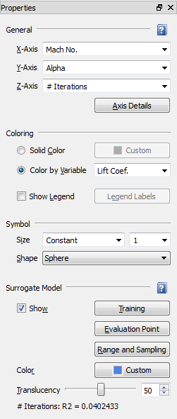
In Tecplot Chorus, the surrogate model may be shown in line plots and in 3D scatter plots. For these plot types, a Surrogate Model section appears in the Properties sidebar containing the controls you will need to train and visualize the model. (The Properties panel shown here is for 3D scatter plots.)

Tecplot Chorus supports a single surrogate model; the same model is used in all plots. However, different variables may be chosen in each plot to visualize different aspects of the model. The range of the input variables and how their values are sampled may also differ among plots.

Training the Model

In the training process, you specify the independent variables (inputs or parameters) to consider, and Tecplot Chorus generates a surrogate model based on correlations between these variables and the dependent variables (outputs or results) in your project.

You train your model via the Surrogate Model Training dialog, which can be accessed from the sidebar for the Line Plot or 3D Scatter Plot by clicking the Training button, or by choosing Surrogate Model → Training from the menu bar.

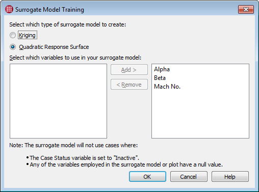
This dialog allows you to choose the type of surrogate model to be generated and to specify the independent variables (inputs or parameters) to be considered by the surrogate model.

Type of model

Choose Kriging or Quadratic Response Surface.

Kriging: A statistical interpolation that yields the best linear unbiased prediction of values between cases using a covariance model (variogram). The more computationally intensive of the two methods, but may produce better results with smaller numbers of cases. A kriging-based model is guaranteed to touch all actual data points (although this may not always be obvious in plots) but may not be as smooth as the alternative.
Quadratic response surface: A simpler least-squares approximation using a second-degree polynomial. A good fit for CFD and other physics applications, as many physical phenomena are at most quadratic. Faster than kriging and generally sufficient for getting "the lay of the land" when the number of cases is too large to wait for kriging.

Independent variables

Choose the independent variables to be used in your surrogate model.

Click a variable in the left column, then click Add >, to move it to the right column and into the surrogate model.
Click a variable in the right column, then click < Remove, to move it to the left column and out of the surrogate model.

You may select multiple variables in either column by holding Control or Shift while clicking, making it easier to add or remove multiple variables from the model. Press Control-A to select all variables in a column.

Click OK to train the surrogate model with the variables you have chosen. Depending on the number of cases in your project, the number of variables included in the model, the model’s type, and your workstation’s performance, this may take anywhere from a few seconds to a few minutes.

A single surrogate model can be active at any one time; the model you create in the Surrogate Model Training dialog is queried to generate the response that may be shown in open Line Plot and 3D Scatter Plot windows. Each of these windows can, however, show the model’s response for a different combination of independent and dependent variables. You can also choose different query values for the input variables in each plot (see Setting Range and Sampling).

Surrogate Model in Line Plots

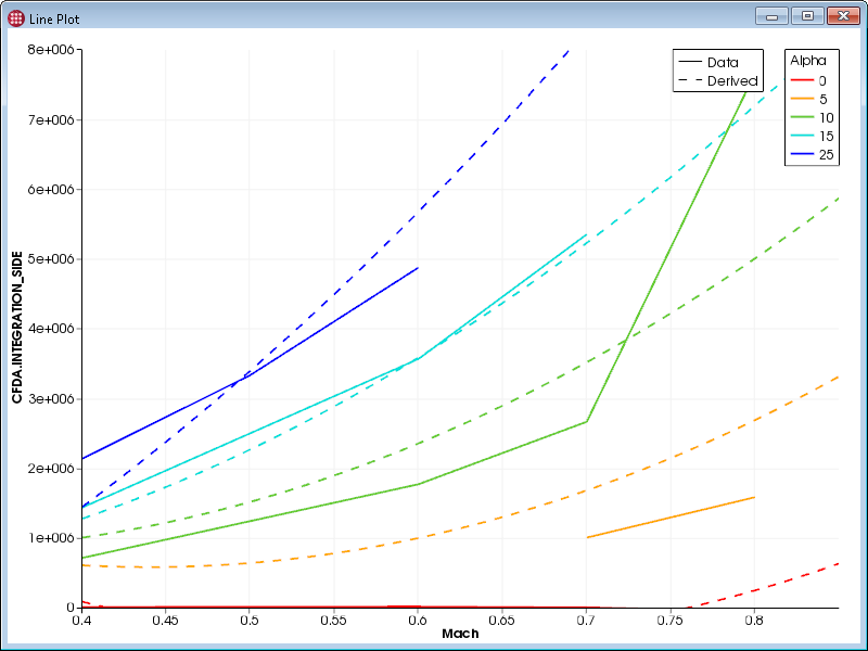
To display surrogate model results on a line plot, the plot must be set up in one the two following ways:

An independent variable on one axis and a dependent variable on the other.
Dependent variables on both axes and one independent variable as Sort By.

Often the X axis will be used for an independent variable and the Y axis for a dependent variable. (See Line and Symbol Plot Properties for details on choosing these variables.)

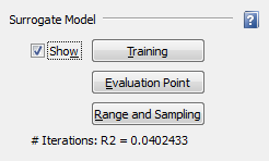
The Properties panel for Line Plots includes the Surrogate Model section, in which the following options are available.

Training: Displays the Surrogate Model Training dialog, described in Training the Model, where you can change the type of surrogate model to generate and the parameters to be included in the model.
Show: Activate this checkbox to see the surrogate model’s prediction on the plot, based on the values of the independent variable used as an axis or as the Sort By variable.

This checkbox is available only after you have trained a surrogate model and chosen appropriate variables as described above.

The response of the surrogate model is displayed as one or more dashed lines. Dashed lines are used even if the plot is set to use symbols or symbols and lines for the actual case values. If multiple lines are shown on the plot (due to the plot’s Sort By setting), multiple dashed lines are shown. The color of each dashed line matches the color of the corresponding solid line representing your actual results.

It may take a moment to query the model and display the result, and the model needs to be re-queried when the plot’s variables are changed. When you are not actively using the surrogate model, turn off this checkbox to avoid these delays. If the wait is excessive, you might consider querying the model at fewer points by Setting Range and Sampling.
Evaluation Point: Opens a dialog (see Setting the Evaluation Point) to specify the query value for the independent variables being used in the surrogate model that are not being used on the plot.
Range and Sampling: Opens a dialog (see Setting Range and Sampling) to choose ranges and the number of query values to use for the independent variable(s) used in the plot.

At the bottom of the panel is an R-squared coefficient of determination indicating the goodness of fit of the surrogate model to the actual data for the dependent variable(s) currently displayed on the plot. The closer R-squared is to 1.0, the better the fit is.

Exporting Derived Data from a Line Plot

To export the values calculated by a surrogate model as a CSV file, the surrogate model response must be visible on the plot. Right-click the plot and choose Export Derived Data from the context menu. A Save dialog appears to let you name the file and choose the folder where it will be saved.

The exported file normally includes results for an evenly-spaced distribution of the independent variable’s range (or the actual values when the independent variable is the Sort By variable). Other input variables are, by default, queried at the minimum value found in the project for that variable.

Often, you will want to export derived data for points that are not in the project to answer questions like "what does the surrogate model predict that the lift coefficient would be at with a value of Alpha for which I have not run a simulation?" The Range and Sampling dialog (see Setting Range and Sampling) can be used to override the default query values for the plot’s independent variable. The Evaluation Point dialog (see Setting the Evaluation Point) can be used to change the query value for other independent variables.

Surrogate Model in 3D Scatter Plots

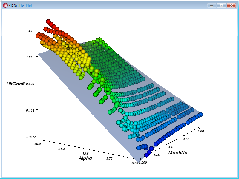
To display surrogate model results on a 3D scatter plot, the plot must employ exactly two independent variables. These variables can be used either on two of the three axes, or as the Color By and Size variables.

Often the X and Y axes are used for independent variables, and the Z axis for an independent variable, as shown above. (See 3D Scatter Plot Properties for details on choosing these variables.)

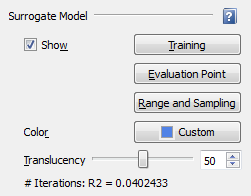
The Properties panel for 3D Scatter Plots includes the Surrogate Model section, in which the following options are available.

Training: Displays the Surrogate Model Training dialog, described in Training the Model, where you can change the type of surrogate model to generate and the parameters to include in the model.
Show: Activate this checkbox to visualize the surrogate model’s prediction for the dependent variable on the plot, based on the values of the two independent variables.

This checkbox is available only after you have trained a surrogate model and assigned appropriate variables as described above. The surrogate model’s response is displayed as a translucent blue surface in the plot by default (both the color and the translucency can be changed).

It may take a moment to query the model and display the result, and the model needs to be re-queried when the plot’s variables are changed. When you are not actively using the surrogate model, turn off this checkbox to avoid these delays. If the wait is excessive, you might consider querying the model at fewer points by Setting Range and Sampling.
Evaluation Point: Opens a dialog (see Setting the Evaluation Point) to optionally specify a single value for each independent variable being used as input to the surrogate model but not being used in the plot.
Range and Sampling: Opens a dialog (see Setting Range and Sampling) to choose ranges and the number of query values to use for each independent variable.
Color: Choose the color for the surface representing the derived data by picking a swatch. Choose the … color swatch to select any color using a standard color picker dialog.
Translucency: Choose the level of translucency for the surrogate model surface using the slider. 0 is opaque and 100 is fully transparent. You may also enter a numeric value directly, or use the small arrow buttons to fine-tune the value.

At the bottom of the panel is an R-squared coefficient of determination indicating the goodness of fit of the surrogate model to the actual data for the displayed dependent variable(s). The closer R-squared is to 1.0, the better the fit is.

Exporting Derived Data from a 3D Scatter Plot

To export the values calculated by a surrogate model as a CSV file, the surrogate model must be active. Right-click the plot and choose Export Derived Data from the context menu. A Save dialog appears to let you name the file and choose the folder where it will be saved.

The exported file normally includes results for an even distribution of query values along the axes (if the independent variables are being used in the plot’s axes) or the actual values in the project (if the independent variables are being used to size and color the scatter symbols). Other input variables are, by default, queried at their minimum project value.

Often, you will want to export derived data for values that are not in the project to answer questions like "what does the surrogate model predict that the lift coefficient would be at a combination of Mach, Alpha, and Beta for which I have not run a simulation?" The Range and Sampling button (see Setting Range and Sampling) and the Evaluation Point button (see Setting the Evaluation Point) can be used to override the values of the inputs to the model.

Exporting Surface Coefficients from a 3D Scatter Plot

Right-click a 3D scatter plot while a response surface surrogate model is active and choose Export Surface Coefficients from the context menu to produce a text file showing how the model calculates the dependent variable value. This file may be viewed in any text editor, such as Notepad.exe on Windows.

An example of this file is shown below.

Independent Variables

V1 = Alpha
V2 = Beta
V3 = Mach

Equation for dependent variable: Drag

Result = 575144 + 2021.56*V1 + -145.074*V1**2 + 9443.39*V2 +
-213.566*V2**2 + -2.33378e+006*V3 + 2.54697e+006*V3**2 + 466.728*V1*V2 +
-14425.1*V1*V3 + -15397.4*V2*V3

Setting the Evaluation Point

For each independent variable that is used as an input to the surrogate model, but which is not being used on the plot, the default query value of that variable is the lowest value of the variable available in your project at the time of model training.

If an independent variable is being used on a plot, multiple values for that variable are used for surrogate model queries. See Setting Range and Sampling.

To change this behavior, click the Evaluation Point button in the Surrogate Model section of the plot’s Properties sidebar, or choose Surrogate Model → Evaluation Point from the menu bar. The Surrogate Model Evaluation Point dialog appears. (If you have not yet trained a model, the Surrogate Model Training dialog appears first.)

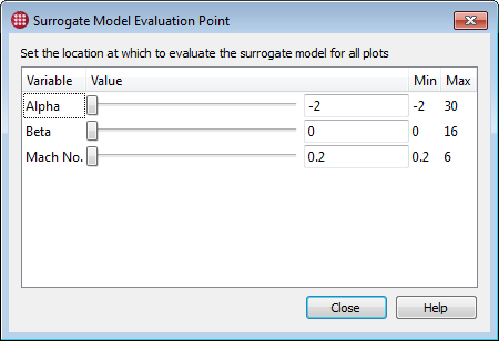
The Surrogate Model Evaluation Point dialog allows you to choose a single value for each input being considered by the model.

Use the slider to select the query value to be used for each variable, or enter a value directly in the text field. The slider respects the minimum and maximum values shown, but you may enter a number outside this range in the text field.

The specified evaluation point is global, and applies to all plots in which the surrogate model is shown. These values are also used when generating derived data (see Exporting Derived Data from a Line Plot and Exporting Derived Data from a 3D Scatter Plot).

Setting the Evaluation Point from a Selected Case

To choose a case’s variable values for the surrogate model, right-click a case in any view or plot, then choose Set Surrogate Model Evaluation Point from the context menu. The Surrogate Model Evaluation Point dialog opens with the selected case’s values filled in for all independent variables used in the model. The new values are applied immediately to all open plots that are currently displaying a surrogate model response. You can then, if desired, fine-tune the values using the sliders and fields in the dialog.

The selected case may not be used as the evaluation point if it has null or NaN values for any model input variable.

Setting Range and Sampling

To calculate a response curve or surface, Tecplot Chorus normally uses query values of the independent variables used in the plot according to the following rules:

Where the variable is used	Default range and sampling
Plot axis	Even distribution within the axis range
Group Data By (in Line Plots)	The actual values of the variable found in the project
Sort By (in Line Plots) Color By (in 3D Plots) Size (in 3D Plots)	Even distribution between the minimum and maximum values found in the project

Where the variable is used

Default range and sampling

Plot axis

Even distribution within the axis range

Group Data By (in Line Plots)

The actual values of the variable found in the project

Sort By (in Line Plots) Color By (in 3D Plots) Size (in 3D Plots)

Even distribution between the minimum and maximum values found in the project

The same query values are used when exporting derived data.

If a variable is not being used in a plot, but is an input to the surrogate model, these rules do not apply. Instead, the evaluation point determines the variable’s query value. See Setting the Evaluation Point.

You can change these behaviors by specifying your own range and sampling instructions for the plot’s independent variables. The specified values are then used as the values of the associated variable when querying the model. You can use this feature both to limit the extent of the surrogate model response shown on the plot and to choose the query values for exports.

Click the Range and Sampling button in the Surrogate Model section of a Line Plot’s or 3D Scatter Plot’s Properties panel. The Surrogate Model Range and Sampling dialog appears.

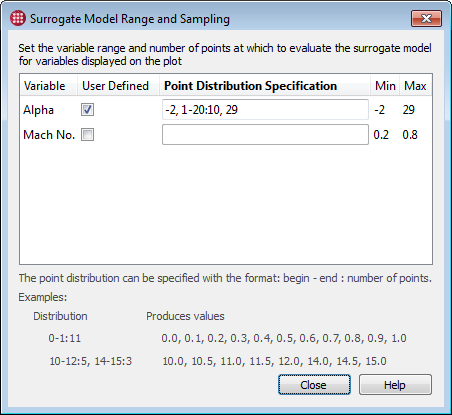
The Surrogate Model Range and Sampling dialog allows you to specify ranges for model input variables used in the active plot as well as how many query values will be distributed across each range. Either one or two variables are displayed depending on whether the active plot is a line plot or a 3D scatter plot. Mark the User Defined checkbox next to the variable of interest and specify values as a comma-separated list of exact values and/or ranges.

A range is specified in the format first-last:samples; that is, the first value in the range, followed by a hyphen, followed by the last value in the range, followed by a colon, followed by the number of equally-spaced samples to take from the range. The range is inclusive of the specified first and last values. For example, 0-1:11 specifies the eleven values 0.0, 0.1, 0.2, 0.3, 0.4, 0.5, 0.6, 0.7, 0.8. 0.9, and 1.0.

Single values and ranges may be combined in any order. For example, 5, 6, 7, 8, 10-15:6, 20-25:6 specifies the values 5, 6, 7, 8, 10, 11, 12, 13, 14, 15, 20, 21, 22, 23, 24, and 25.

The line or surface displayed in your plot, which represents the surrogate model’s response, respects the minimum and maximum of the values specified in this dialog. The model is queried at the exact points specified (for 3D plots, all combinations of the points specified when the independent variables are being used as axes), both for drawing the model’s response on plots and for exporting derived data; see Exporting Derived Data from a Line Plot and Exporting Derived Data from a 3D Scatter Plot.