21 - 4 Setting Geometry and Boundary Options
For certain calculations, you will need to specify information about your data that Tecplot 360 EX may not automatically detect. For example, a 2D solution may actually represent a 3D axisymmetric solution, affecting any integrations you perform. Adjacent zones may be connected, affecting other calculations such as grid stretch factors, gradients, and flow features such as vortex cores. Certain zones or zone surface regions may represent wall boundaries in your solution, on which separation and attachment lines may be calculated. The FLUENT data loader identifies most of these characteristics for you when you import FLUENT case and data files. You may also specify them with the Geometry and Boundaries dialog (accessed via the Analyze menu).
For a layout with multiple datasets, separate settings are maintained for each dataset. You can copy the settings from one dataset to another using the Save Settings and Load Settings options in the Analyze menu. These actions also transfer the settings made in the Fluid Properties, Reference Values, Field Variables, and Unsteady Flow Options dialogs.
You must have data in the active frame to launch the Geometry and Boundaries dialog. Select "Geometry and Boundaries" from the Analyze menu to display the dialog.
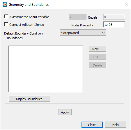
• Specifying an Axisymmetric Solution - Selecting Axisymmetric About Variable enables the Variable drop-down menu and allows you to enter a value in the Equals field. Select X or Y from the Variable drop-down, and enter the constant value of this variable that defines the axis of symmetry. If you choose the axisymmetric option, all integrations will be performed as 3D axisymmetric integrations by multiplying the integrand by  , where r is the distance from the specified axis of symmetry. Integrations are described in Section 21 - 7 “Performing Integrations”.
• Connecting Adjacent Zones - Tecplot 360 EX can calculate whether nodes on the boundaries of adjacent zones (or the same zone) overlap. It uses this information in calculating the Stretch Ratio grid quality function (see Section G - 2.2 “I, J, or K-stretch Ratio”), calculating gradients, and extracting fluid flow features (see Section 21 - 11 “Extracting Fluid Flow Features”). Connections between zones are calculated cell face by cell face. The two cells are considered connected wherever all nodes of a particular boundary cell face overlap all nodes of an adjacent boundary cell face.
For unsteady flows (see Section 21 - 5 “Unsteady Flow”), only zones within the same time level are examined for connections. To enable this option, select the Connect Adjacent Zones option and enter the maximum distance at which two nodes will be considered to overlap in the Nodal Proximity text field. Note that this text field value is also used for zone-type boundaries, discussed below.
The zone connection feature is overridden, cell-by-cell, by any face neighbors contained in a dataset. Both connection mechanisms are overridden by any boundary conditions set on a particular face. That is, if you specify a boundary condition in the Geometry and Boundaries dialog that covers a specific cell face, that face will not be connected to an adjacent cell, irrespective of any face neighbors or overlapping nodes present.
21 - 4.1 Performance Considerations
Establishing connections across zone boundaries allows Tecplot 360 EX to calculate better gradient quantities at these locations. There may be a substantial performance penalty for ordered-zone calculations, because at these boundary locations, Tecplot 360 EX uses the finite element least-squares formulation for calculating the gradients. Refer to Section 21 - 6.5 “Gradient Calculations” for a discussion of gradient calculations.
21 - 4.2 Specifying Boundaries and Boundary Conditions
You may associate cell boundary faces (cell faces on the exterior of a zone) with a boundary condition. There are two reasons why you might want to do this:
• To ensure that boundary faces are not connected to adjacent cells (see the above discussion on connections).
• To identify wall boundaries in 3D solutions for feature extraction (see Section 21 - 11 “Extracting Fluid Flow Features”).
If you set a boundary condition on a particular cell boundary face, that face will not be considered connected to any other cells by the gradient calculation routines. This may be advantageous, for example, in solutions containing a thin flat plate, where nodes on either side of the flat plate overlap and would otherwise be connected by the connection mechanism.
For three-dimensional flow solutions, you can use the Extract Flow Features dialog to extract separation and attachment lines. These lines are only calculated on boundaries you have identified as wall boundaries. While other boundary conditions may be specified, this information is not currently used, aside from inhibiting connections.
Specifying the Default Boundary Condition
Tecplot 360 EX keeps track of all unconnected boundary cell faces (see Section 21 - 4 “Setting Geometry and Boundary Options”) It applies the default boundary condition to any unconnected faces to which you do not specifically apply a boundary as described below. Choose the desired boundary condition from the Default Boundary Condition drop-down. The default boundary condition is at the bottom of the boundary 'pecking order.' If a cell boundary face is not covered by any other boundary condition, and is not connected to any other cells by either Geometry and Boundaries connection settings or Tecplot 360 EX face neighbors, then the default boundary condition is applied to it.
Regions on the boundaries of zones may be explicitly identified and associated with particular boundary conditions. For ordered zones only, you may identify a boundary region by zone boundary (that is, the I=1 boundary) and index range on that boundary. For all zone types, you may identify a boundary region by selecting one or more boundary zones.
Boundary zones are zones of dimension one less than the current plot type. They are surfaces in 3D Cartesian plots, or lines in 2D Cartesian plots. Boundaries are considered to exist wherever the nodes of these boundary zones coincide with nodes on the boundaries of volume zones in 3D Cartesian plots, or surfaces in 2D Cartesian plots. For example, you can identify boundary regions on a tetrahedral (3D) zone using triangular zones that lie on the surface of the tetrahedral zone. The boundary is applied wherever the nodes of the triangular zone overlap boundary nodes of the tetrahedral zone. As with connecting adjacent zones, the matching is done cell face by cell face using the Nodal Proximity setting of the Geometry and Boundaries dialog to determine how close to each other nodes must be to be considered overlapping.
It is easy to create boundary zones by extracting subzones from ordered zones in your dataset. For finite element zones, it may be possible to extract the desired boundary region using blanking and FE-boundary extraction. In general, however, finite element boundary zones must come from your grid generator or flow solver.
New boundaries are created by clicking New on the Geometry and Boundaries dialog. This displays The Edit Boundary dialog, shown below.
Displaying Boundaries
The current settings of the Geometry and Boundaries dialog may be displayed by clicking the [Display Boundaries] button. This creates a new frame and plots all zone boundaries. For each zone in your solution data, one zone will be created in the new frame for each boundary condition applied to the boundary faces of that zone. The names of these zones indicate their zone of origin in your solution data and the applied boundary condition.
For each boundary face in your solution, Tecplot 360 EX applies some simple rules to determine that face's boundary condition. First, all faces covered by the boundary definitions in the Boundaries list have the boundary conditions prescribed in the list applied to them. If a particular face is covered by more than one of these boundaries, the boundary lowest in the list takes precedence. If you have selected the Connect Adjacent Zones option, any faces not covered by the listed boundaries are then checked to see if they overlap faces of neighboring zones. Overlapping faces are assigned the boundary condition 'Interzone Boundary.' Finally, any boundary faces not assigned any other boundary condition will be assigned the default boundary condition you have chosen.
Since the Geometry and Boundaries dialog is modeless, you can explore the boundary definitions in this new frame prior to applying your settings. This is a convenient way to make sure you are applying the desired boundary settings.
Selecting the [Display Boundaries] button records a DISPLAYBOUNDARIES macro command if you are recording a macro file.
Since this feature creates a new frame, it cannot be saved in the data journal, and the current data journal is invalidated. If you subsequently save a layout file, you will be prompted to save a new data file.
Saving Geometry and Boundary Settings
Once you are satisfied with your geometry and boundary settings, you can save them by selecting the [Apply] button. When you apply your settings, a SETGEOMETRYANDBOUNDARIES macro is recorded (if you are recording a macro file).