21 - 6.4   Selecting a Function

The function name may be typed into the Name text field, or selected from a list which contains all available functions. Click [Select] to display the Select Function dialog.

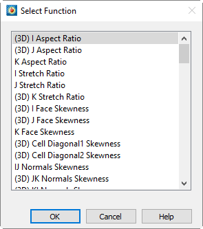
Selecting a function from this dialog and selecting [OK] enters that function in the appropriate area. Functions in this list which only apply to 3D solution data begin with (3D). Vector functions, whose names are appended with (vector), calculate three vector components. Each of the available functions is described in Chapter G: “Calculate Variables Reference”.

An alternative method of selecting a function is to enter its equivalent PLOT3D function number. These numbers may also be found in Chapter G: “Calculate Variables Reference”. If a valid function number is entered into the Name text field in the Calculate dialog, Tecplot 360 EX replaces the number with the name of the corresponding function and sets the Normalize drop-down to None or Reference Values as appropriate.

21 - 6.5   Gradient Calculations

Most of the PLOT3D functions are scalar functions. Gradient calculations are a notable exception to this rule, however, and depend on values at neighboring points. Understanding how these calculations are performed may help you interpret the results.

Gradients in Ordered Zones

With an exception for boundary nodes discussed below, gradients in ordered zones are calculated using standard finite-difference formulae. To calculate pressure gradient at a particular node in an ordered zone, for example, the following formula is used:

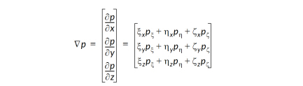
Where x indicates the I-direction, h indicates the J-direction, z indicates the K-direction and subscripts indicate partial derivatives. In the zone interior, derivatives are estimated with second-order central differences, such as:

The left-hand form is used for calculating gradients at nodes, and the right-hand form is used at cell centers.

Boundary nodes of ordered zones that are not part of a boundary specified in the Geometry and Boundaries dialog are first examined to see whether they lie on a boundary face connected to other cells via face neighbors. If not, and if the "Connect Adjacent Zones" option is set in the Geometry and Boundaries dialog, the node is examined to determine if its location coincides with any boundary nodes of adjacent zones. If either is the case, the gradients for that node is calculated using the method described below for finite element zones. Otherwise, its gradients are calculated using standard one-sided (first-order) finite differences.

Gradients in Finite Element Zones

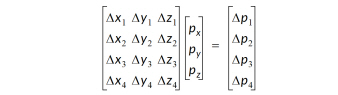
The coordinate transformation approach used in unconnected ordered zones is generally not possible for finite element zones. Instead, the variable, say pressure, is assumed to vary linearly in all dimensions, giving:

where p₀ is the pressure at the node or cell center in question. Next, a matrix equation is formed with the pressure difference for all nodes neighboring the current node (see below for how these neighboring nodes are found).

To reduce the influence of nodes far away from the value being calculated, each row i of this matrix equation is scaled by:

 

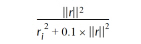
Where r_i is the distance from node i to the target location (node or cell center) and:

 

This equation is generally over-specified and is inverted by least-squares to find the gradient vector.

If the cell-centered gradient is being calculated, each row in the above matrix equation is calculated from the values at the nodes that comprise the cell. If a node-centered gradient is being calculated, all nodes connected to that node by a cell edge are used. If the node lies on a zone boundary and is not covered by a boundary specified in the Geometry and Boundaries dialog, two additional steps are taken to give more continuous gradients across the zone boundary:

1.If the node is part of a face connected to other cells by face neighbors, then the nodes of those neighboring cells are also used;

2.Otherwise, if the "Connect Adjacent Zones" option is enabled in the Geometry and Boundaries dialog, the node is examined to see if its location coincides with a boundary node in an adjacent zone. If so, all nodes connected to that node by a cell edge are also used.

21 - 6.6   Surface Normal Calculations

With Tecplot 360 EX's CFDA variable calculation feature, you can calculate and display surface normal vectors on your plot. This includes the following steps:

1.With the Calculate dialog, calculate the "Grid K Unit Normal (vector)", using Cell Center as the New Var Location.

2.Turn on the Vector layer, selecting the components of the vector you just calculated as the vector components.

3.In the Zone Style dialog, on the Points page, choose "Cell Centers Near Surfaces" as the Points to Plot.

In detail, the steps above include the following.

To calculate the normal, choose "Calculate Variables" from the Analyze menu. In the Calculate dialog, choose "Grid K Unit Normal (vector)" as the variable to calculate (to do this, click the Select button, and scroll down in the list that appears to find "Grid K Unit Normal (vector)", and click it). Choose "Cell Center" as the New Var Location, and click Calculate.

Next, toggle-on the Vector layer in the Plot sidebar to turn on the normal vectors, and choose the components of the calculated vector to display in the Select Variables dialog for vectors. This dialog appears when you toggle-on the vector layer for the first time; you can also open the dialog by going to Plot > Vector > Variables in the menu bar. To display the "Grid K Unit Normal (vector)" normal, choose the three components "X Grid K Unit Normal", "Y Grid K Unit Normal", and "Z Grid K Unit Normal" for the X, Y, and Z components of the vector layer, respectively.

Lastly, click the Zone Style button in the Plot sidebar to open the Zone Style dialog. In that dialog, switch to the Points page, and choose "Cell Centers Near Surfaces" from the Points to Plot menu.