Tensor Eigensystem

31 - 3.13 Tensor Eigensystem

The Tensor Eigensystem add-on loads automatically with Tecplot 360 EX. This add-on enables you to calculate the eigenvalues and eigenvectors of a 3-by-3 symmetric tensor whose components are stored in your data set. The add-on calculates for each node in the data set and stores the results as new data set variables.

To use this add-on, select "Tensor Eigensystem" from the Tools menu to open the Tensor Tools dialog. To unload the add-on, comment out the line including the libname "tecutiltools_tensoregn" in your Tecplot.add File.

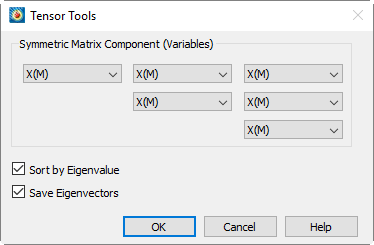
In the Tensor Tools dialog, select variables from your data set to represent the 6 components of the tensor. Toggle-on "Sort by Eigenvalue" to sort the results by the eigenvalues, and/or toggle-on "Save Eigenvectors" to store the calculated eigenvectors in addition to the calculated eigenvalues, which the calculation always saves. Then select [OK] to perform the calculation.

Tecplot 360 EX will store the eigenvalues of the tensor as variables EgnVal1, EgnVal2, and EgnVal3 in your data set. If you choose to save the eigenvectors as well, they are stored as variables EgnVec11 through EgnVec33. If you toggled-on "Sort by Eigenvalue", the eigenvalues and their corresponding eigenvectors will be sorted largest-to-smallest at each grid node. The association of EigenValue to EigenVector is as follows:

EigVal1 ---> EgnVec11, EgnVec21, EgnVec31

EigVal2 ---> EgnVec12, EgnVec22, EgnVec32

EigVal3 ---> EgnVec13, EgnVec23, EgnVec33

A common use of Tensor Eigensystem is to visualize vortex cores in a flow solution. You can do this by the following method:

1.Calculate Velocity Gradient in Analyze>Calculate Variables

2.Calculate the symmetric tensor S2 + Ohm-2 with Data>Alter>Specify Equations (see below for an equation file to perform this)

3.Use the Tensor Eigensystem dialog to calculate the sorted eigenvalues

4.Display an iso-surface of Lambda-2, the middle of the three eigenvalues, which is negative in the vicinity of a vortex core

The following equation file calculates the required symmetric tensor components of S2 + Ohm-2 from the velocity gradient for step 2 above. Save the below to a text file, then load it into the Specify Equations dialog by selecting "Load Equations" and selecting the file.

#!MC 1100

$!ALTERDATA EQUATION = '{s11} = {dUdX}'

$!ALTERDATA EQUATION = '{s12} = 0.5*({dUdY}+{dVdX})'

$!ALTERDATA EQUATION = '{s13} = 0.5*({dUdZ}+{dWdX})'

$!ALTERDATA EQUATION = '{s22} = {dVdY}'

$!ALTERDATA EQUATION = '{s23} = 0.5*({dVdZ}+{dWdY})'

$!ALTERDATA EQUATION = '{s33} = {dWdZ}'

$!ALTERDATA EQUATION = '{Omga12} = 0.5*({dUdY}-{dVdX})'

$!ALTERDATA EQUATION = '{Omga13} = 0.5*({dUdZ}-{dWdX})'

$!ALTERDATA EQUATION = '{Omga23} = 0.5*({dVdZ}-{dWdY})'

$!ALTERDATA EQUATION = '{s2o2_11} = {s11}**2 + {s12}**2 + {s13}**2 - {Omga12}**2 - {Omga13}**2'

$!ALTERDATA EQUATION = '{s2o2_12} = {s11}*{s12} + {s12}*{s22} + {s13}*{s23} - {Omga13}*{Omga23}'

$!ALTERDATA EQUATION = '{s2o2_13} = {s11}*{s13} + {s12}*{s23} + {s13}*{s33} - {Omga12}*{Omga23}'

$!ALTERDATA EQUATION = '{s2o2_22} = {s12}**2 + {s22}**2 + {s23}**2 - {Omga12}**2 - {Omga23}**2'

$!ALTERDATA EQUATION = '{s2o2_23} = {s12}*{s13} + {s22}*{s23} + {s23}*{s33} - {Omga12}*{Omga13}'

$!ALTERDATA EQUATION = '{s2o2_33} = {s13}**2 + {s23}**2 + {s33}**2 - {Omga13}**2 - {Omga23}**2'

Remember that the Tensor Eigensystem add-on can only analyze 3-by-3 symmetric tensors (not 2-by-2, anti-symmetric, or non-symmetric tensors).

Macro Processing

To invoke the tensor eigensystem add-on with a macro, use the following syntax.

$!EXTENDEDCOMMAND

COMMANDPROCESSORID = 'Tensor Eigensystem'

COMMAND = 'T11VarNum = <varref>\nT12VarNum = <varref>\nT13VarNum = <varref>\nT22VarNum = <varref>\nT23VarNum = <varref>\nT33VarNum = <varref>\nSortEgnV = <Boolean>\nSaveEgnVect = <Boolean>'

Where <varref> can be an integer or the variable name contained within double quotes.

31 - 3.14 Time Series

The Time Series add-on, libname "tecutiltools_timeseries," loads automatically with Tecplot 360 EX. It extracts a single point over time and plots the result in a new frame as an XY Line Plot. The solution time of the time series plot's frame is linked to that of its parent, and a marker gridline is added to show the current solution time. If a nearest-point probe is performed (using Control-click), you may follow a particular node through time, or through an XY(Z) location.

When tracking a node through time, each zone must have the same node map (or a shared node map).

This add-on may not work as expected when there are multiple zones in the same strand at the same solution time.

To use the Time Series add-on, choose one of the following menu options from the Tools menu:

• Probe To Create Time Series Plot - This option sets the mouse mode to probe. You can use either the mouse or the Probe At dialog to probe a point. The probed location will be sampled over time (for transient data) and a resulting XY Line Plot will be created. If a nearest point probe is done (Control-click), a dialog appears to ask if you want to track the node or the XY(Z) location through time. If you track the node, it is important that your data has the same node map for each zone through time.

• Send Time Series Data To New Frame - This option creates a new frame for each point extracted. By default, the frame used for the time series data is reused to avoid creating an excess of frames.