21 - 9   Calculating Particle Paths and Streaklines

For steady-state solutions, Tecplot 360 EX allows you to track the paths of massless particles by placing streamtraces in the flow. The Particle Paths and Streaklines dialog augments this capability by providing two additional visualization methods, particle paths and streaklines, for particles with or without mass.

Please note that these calculations, particularly for streaklines, may be very lengthy to perform, especially for cases with large grids.

The Particle Paths and Streaklines dialog is displayed by selecting Calculate Particle Paths and Streaklines from the Analyze menu.

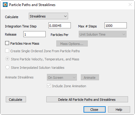
It contains a drop-down menu allowing you to choose particle paths or streaklines, as well as options pertaining to the path integrations, particles with mass, storage and display of the calculated particle paths. In addition, the results of streaklines may be animated.

21 - 9.1   Calculating Particle Paths

A particle path is the path that a single particle follows through a solution. In steady flow, particle paths are the same as streaklines and streamtraces for massless particles. To calculate particle paths, you must:

1.Place streamtraces at the locations where you wish particles to be released, then select Particle Paths from the drop-down menu at the top of the dialog. (Details on placing streamtraces may be found in the Chapter 15: “Streamtraces”.)

2.Specify an integration time step. For steady-state calculations, specify the maximum number of time steps to be performed (see Section 21 - 5 “Unsteady Flow” for specifying steady or unsteady flow).

3.Set the Particles Have Mass option for particles with mass. Click Mass Options to set mass-related options.

4.Optionally, set the Create Single Ordered Zone From Particle Paths toggle to create a single IJ-ordered zone from all particle paths instead of a separate I-ordered zone from each path.

5.Select [Calculate].

Specifying the Integration Time Step and Maximum Number of Steps

Particle Paths are calculated by integrating the velocity field of your solution using a constant time step, which you enter in the Integration Time Step text field. A smaller time step will result in more accurate particle paths but will take longer to calculate. For unsteady calculations, the time step is set equal to the time interval between your solution time levels by default. If you specify so large a time step that a particle passes out of your solution domain in the first integration time step, you will get a warning message.

If you have set the Flow Solution is Steady-state option, you must also enter the maximum number of integration time steps to be performed (see also Unsteady Flow).

Specifying Mass-Related Options

For particles with mass, set the Particles Have Mass option. This enables other mass-related controls in the dialog. Click Mass Options to display the Particle Mass Options dialog. (See Section 21 - 9.3 “Particles with Mass”) In addition, you have the option of storing the particle's velocity and other particle properties or the local flow properties along the calculated particle path. Select Store Particle Velocity, Temperature, and Mass to store these values along the particle path. Select Store Interpolated Solution Variables to store these values instead. Following the calculation, you will be informed of which dataset variables contain these values.

Performing the Particle Path Calculation

When you select Calculate, a particle is placed at the starting point for each streamtrace you have placed. If you did not place any streamtraces, you will get an error message. From these starting locations, beginning with the time equal to the time of your first solution time level (or zero for steady-state calculations), the particle positions are advanced by performing a second-order Runge-Kutta integration of the velocity field. For unsteady calculations, linear interpolation is performed between solution time levels. Integration for each particle is continued until the final time level is reached (unsteady calculations), the specified number of time steps has been performed (steady-state calculations), or until the particle passes out of your solution domain. The particle paths are displayed as new I-ordered zones in your dataset, with each integration step represented by a node in the new zones, unless you selected the Create Single Zone From Particle Paths option, which results in a single IJ-ordered zone.

Examining the Particle Paths

Each I-ordered zone created by a Particle Path calculation represents a path through space and time. The paths' non-grid variables will hold interpolated values of your solution data that the particle "saw" as it passed through your solution, except as discussed in Specifying Mass-Related Options. You can visualize this by coloring the particle zones' mesh plots with one of your solution variables. The following steps will accomplish this:

1.Turn on the Mesh plot layer by toggling-on the Mesh in the Plot sidebar.

2.Call up the Zone Style dialog (accessed via the Plot menu or the Plot sidebar).

3.Turn off mesh plotting for your solution zones by selecting the solution zones, clicking Mesh Show and selecting No.

4.If necessary, turn on mesh plotting for the Particle Path zones by selecting them, clicking Mesh Show and selecting Yes.

5.Color the Particle Path zones with a variable by selecting these zones, clicking Mesh Color and selecting Multi-color. If you had not previously chosen a contour variable, the Contour Variable dialog will open to allow you to select it. Choose the variable you wish to use to color the particle paths.

6.If Auto Redraw has not been selected, click Redraw to redraw your plot. You will see the particle paths displayed and colored with the contour variable.

You may wish to turn on the Scatter plot layer to see the size of these steps. If you do this, you will first want to turn off scatter plotting for your solution zones. You can also do this with the Zone Style dialog.

21 - 9.2   Calculating Streaklines

Streaklines simulate experimental techniques which involve the periodic or continuous release of a tracer substance, such as oil drops or smoke. Tecplot 360 EX produces streaklines by releasing a sequence of particles from the release points and integrating the unsteady velocity field to find their positions in the flow at the end solution time. The final positions of all particles emitted from a particular release point form one streakline. Once streaklines have been calculated, they may be animated on screen or to a file.

To calculate Streaklines, perform the following actions:

1.Identify the solution time levels in your dataset. (See Section 21 - 5 “Unsteady Flow”.)

2.Place streamtraces at the locations where you wish particles to be released.

3.Select Streaklines from the drop-down menu at the top of the Particle Paths and Streaklines dialog.

4.Enter the integration time step as with particle path calculations. (See Specifying the Integration Time Step and Maximum Number of Steps).

5.Specify the particle release frequency. (See Specifying the Particle Release Frequency.)

6.For particles with mass, set the Particles Have Mass option. Click Mass Options to set mass-related options.

7.Select [Calculate].

It is not reasonable to calculate streaklines for steady-state flow, because in steady-state flow, even for particles with mass, streaklines are the same as particle paths (just more time consuming to compute).

Specifying the Particle Release Frequency

For Streakline calculations, a sequence of particles is released throughout the solution time. Each particle's position is integrated using the specified integration time step. The frequency with which particles are released is specified by the controls just above the [Calculate] button. In the Release text field, enter the number of particles to be released in the specified time interval. In the particles per drop-down menu, identify this time interval by selecting either Solution Time Level or Unit Solution Time.

If you select Solution Time Level, the indicated number of particles will be released, evenly spaced in time, between each pair of solution time levels you have identified. If you select Unit Solution Time, the particles will be released at regular intervals throughout the time covered by your solution. In either case, a particle will be released at the final time of your solution, so that the streaklines will include the release points themselves. Releasing particles more frequently will produce more detailed streaklines (the accuracy is determined by the Integration Time Step), but will take longer to calculate.

Performing the Streakline Calculation

When you click Calculate, the streaklines are calculated and added to your dataset as new I-ordered zones. To see them, turn on the Mesh plot layer and disable mesh plotting for your solution zones. See Examining the Particle Paths.

Animating Streaklines

Once you have performed a streakline calculation, the animation controls of the Particle Paths and Streaklines dialog are enabled. A streakline animation displays each successive step in the integration, and can be an effective means of visualizing the unsteadiness of a flow. Toggle-on Include Zone Animation in the Particle Paths and Streaklines dialog to animate the zones along with the streaklines.

 

You may display the animation in the frame in which the streaklines were calculated or save it to a video file in a number of formats. To perform a streakline animation, perform the following steps:

1.Delete the I-ordered zones of any streaklines you do not wish to be part of the animation using Data>Delete>Zone.

2.Select the animation destination from the Animate Streaklines dropdown.

3.Select Animate.

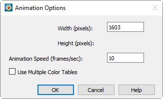
4.If you chose to save the animation to a file, the Animate Options dialog will be displayed. Enter your choices for the animation and select [OK]. Then choose a file name in the resulting file selection dialog.

While animating on the screen, the [Animate] button's text will change to Cancel, allowing you to stop the animation. While animating to a file, a progress dialog will be displayed that allows you to cancel the animation.

Deleting Particle Paths and Streaklines

Particle paths and streaklines are saved either as I-ordered zones or as a single IJ-ordered zone. You may delete these individually using the Delete Zone dialog (accessed via Data>Delete>Zone). If you wish to delete all previously calculated particle paths and streaklines, you may do so using the [Delete All Particle Paths and Streaklines] button. This deletes all zones whose names begin with 'Particle Path' or 'Streakline.'