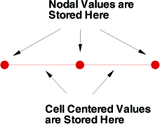
Ordered data is defined by one, two, or three-dimensional logical arrays, dimensioned by IMAX, JMAX, and KMAX. These arrays define the interconnections between nodes and cells. The variables can be either nodal or cell-centered. Nodal variables are stored at the nodes; cell-centered values are stored within the cells.
• One-dimensional Ordered Data (I-ordered, J-ordered, or K-ordered)
|
|
A single dimensional array where either IMAX, JMAX or KMAX is greater than or equal to one, and the others are equal to one. For nodal data, the number of stored values is equal to IMAX * JMAX * KMAX. For cell-centered I-ordered data (where IMAX is greater than one, and JMAX and KMAX are equal to one), the number of stored values is (IMAX-1) - similarly for J-ordered and K-ordered data.
|
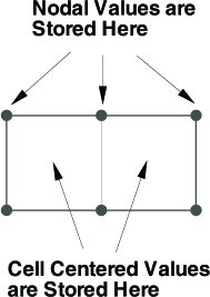
• Two-dimensional Ordered Data (IJ-ordered, JK-ordered, IK-ordered)
|
|
A two-dimensional array where two of the three dimensions (IMAX, JMAX, KMAX) are greater than one, and the other dimension is equal to one. For nodal data, the number of stored values is equal to IMAX * JMAX * KMAX. For cell-centered IJ-ordered data (where IMAX and JMAX are greater than one, and KMAX is equal to one), the number of stored values is (IMAX-1)(JMAX-1) - similarly for JK-ordered and IK-ordered data. |
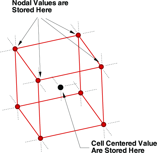
• Three-dimensional Ordered Data (IJK-ordered)
|
|
A three-dimensional array where all IMAX, JMAX and KMAX are each greater than one. For nodal ordered data, the number of nodes is the product of the I-, J-, and K-dimensions. For nodal data, the number of stored values is equal to IMAX * JMAX * KMAX. For cell-centered data, the number of stored values is (IMAX-1)(JMAX-1)(KMAX-1).
|
3 - 2.1 Indexing Nodal Ordered Data
For nodal ordered data, the n-dimensional array of values are treated as a one dimensional array. For example, given an IJK-ordered zone dimensioned by 10x20x30. To access the value at I=3, J=4, K=5 (one based) you would use:
IMax = 10
JMax = 20
KMax = 30
I = 3
J = 4
K = 5
NodeIndex = I + (J-1)*IMax + (K-1)*IMax*JMax
3 - 2.2 Indexing Cell-centered Ordered Data
For cell-centered ordered data, the index that represents the cell center is the same as the nodal index that represents the lowest indexed corner of the cell.
For example, the figure below shows an IJ-ordered zone dimensioned 3x4.
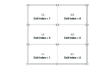
Figure 3-1. An IJ-ordered zone dimensioned 3x4. Cell index numbers are based on the point number in the lowest corner of the cell.
To access a cell-centered value for the cell in the upper right hand corner, use the following:
IMax = 3
JMax = 4
KMax = 1
I = 2
J = 3
K = 1
CellIndex = I + (J-1)*IMax + (K-1)*IMax*JMax
You'll notice that the equations are exactly the same as with nodal data. As a result there are gaps of unused values at IMax, JMax, and KMax that must be left unassigned.
The above equation is generic for 1D, 2D and 3D data. It simplifies for the lower dimensions.
3 - 2.3 One-dimensional Ordered Data (I, J, or K)
Values for XY Line plots are usually arranged in a one-dimensional array indexed by one parameter: I for I-ordered, J for J-ordered, or K for K-ordered, with the two remaining index values equal to one.
At each node, N variables (V1, V2, ..., VN) are defined. If you arrange the data in a table where the values of the variables (N values) at a node are given in a row, and there is one row for each node, the table would appear something like that shown below.
See Chapter 6: “XY and Polar Line Plots” for more information on XY plots.
IJK-ordered Data Plotting
In one or two-dimensional datasets, all data points are typically plotted. However, for IJK-ordered data you can designate which surface will be plotted by using the Surfaces page of the Zone Style dialog. You may choose to plot just outer surfaces, or you may select combinations of I, J, and K-planes to be plotted. Refer to Section 7 - 1.2 “Surfaces” for in-depth information.
3 - 2.4 Logical versus Physical Representation of Data
A family of I-lines results by connecting all of the points with the same I-index, similarly for J-lines and K-lines. For IJ-ordered data, both families of lines are plotted in a two-dimensional coordinate system resulting in a 2D mesh. When both the I and J-lines are plotted in a three-dimensional coordinate system, a 3D surface mesh plot results. An example of both meshes is shown below. As you can see, logical data points can transform into an arbitrary shape in physical space.
|
|
|
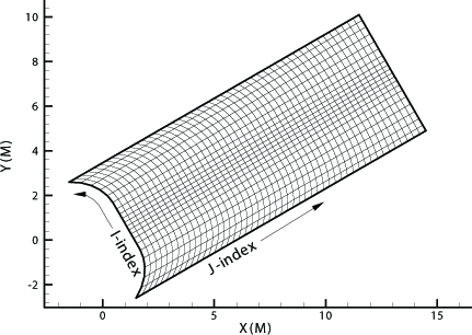
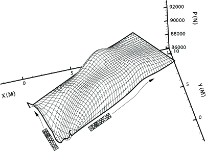
Figure 3-2. Left, a 2D mesh of IJ-ordered data points. Right, a 3D mesh of IJ-ordered data points.