20 - 9.2   Inverse-Distance Interpolation

Inverse-distance interpolation averages the values at the data points from one set of zones (the source zones) to the data points in another zone (the destination zone). The average is weighted by a function of the distance between each source data point to the destination data point. The closer a source data point is to the destination data point, the greater its value is weighted.

In many cases, the source zone is an irregular dataset—an I-ordered set of data points without any mesh structure (a list of points). Inverse-distance interpolation may be used to create a 3D surface or a 3D volume field plots of irregular data. The destination zone can, for example, be a circular or rectangular zone created within Tecplot 360 EX (see “Zone Creation” on page 308).

To perform inverse-distance interpolation in Tecplot 360 EX, use the following steps:

1.Read the dataset to be interpolated into Tecplot 360 EX (the source data).

2.Read in or create the zone onto which the data is to be interpolated (the destination zone).

3.From the Data menu, choose Interpolate>Inverse Distance.

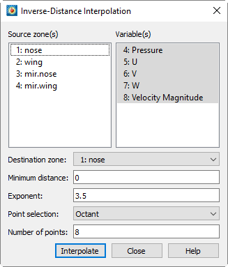
4.From the Inverse-Distance Interpolation dialog, select the zones to be interpolated from those listed in the Source Zone(s) list.

5.Select which variables are to be interpolated from those listed in the Variable(s) list.

6.Select the Destination Zone into which to interpolate. Existing values in the destination zone will be overwritten.

7.[OPTIONAL] Enter the minimum distance used for the inverse-distance weighting in the Minimum Distance text field. Source data points which are closer to a destination data point than this minimum distance are weighted as if they were at the minimum distance. This tends to reduce the peaking and plateauing of the interpolated data near the source data points.

8.[OPTIONAL] Enter the exponent for the inverse-distance weighting in the Exponent text field.

9.[OPTIONAL] Select the method used for determining which source points to consider for each destination point from the Point Selection drop-down. There are three available methods, as follows:

• Nearest N - For each point in the destination zone, consider only the closest n points to the destination point. These n points can come from any of the source zones. This option may speed up processing if n is significantly smaller than the entire number of source points.

• Octant - Like Nearest N above, except the n points are selected by coordinate-system octants. The n points are selected so they are distributed as evenly as possible throughout the eight octants. This reduces the chances of using source points which are all on one side of the destination point.

• All - Consider all points in the source zone(s) for each point in the destination zone.

10. Click Interpolate to perform the interpolation.

 

Inverse-distance interpolation ignores the IJK-mode of IJK-ordered zones. All data points in both the source and destination zones are used in the interpolation.

The Inverse-Distance Algorithm

The algorithm used for inverse-distance interpolation is simple. The value of a variable at a data point in the destination zone is calculated as a function of the selected data points in the source zone (as defined in the Point Selection drop-down, accessed via Data>Interpolate>Inverse-Distance).

The value at each source zone data point is weighted by the inverse of the distance between the source data point and the destination data point (raised to a power) as shown below:

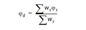(summed over the selected points in the source zone)

where j_d and j_s are the values of the variables at the destination point and the source point, respectively, and w_s is the weighting function defined as:

 

D in the equation above is the distance between the source point and the destination point or the minimum distance specified in the dialog, whichever is greater. E is the exponent specified in the Exponent text field.

Smoothing may improve the data created by inverse-distance interpolation. Smoothing adjusts the values at data points toward the average of the values at neighboring data points, removing peaks, plateaus, and noise from the data. See Section 20 - 2 “Data Smoothing” for information on smoothing.