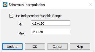
This method of interpolation generates a curve that will never have more inflection points than are clearly required by the given set of data points. The interpolating curve passes through the data points and exactly matches the computed slopes at those points1.
The optional parameters can be accessed by selecting the Curve Settings option on the Curves tab of the Mapping Style dialog.
By default, a series of linear segments are drawn between each set of points for the XY Line plot type.
To turn off curve fits for your data and use linear segments between points:
1.From the Curves page of the Mapping Style dialog, select the mappings you want to show as linear segments.
2.Right-click in the Curve Type column on the Curves page of the Mapping Style dialog and select "Line Segments."
Line Segments are plotted in the order set in the Sort option of the Definitions page of the Mapping Style dialog. By default, the points are unsorted, and lines segments are drawn in the order the data points appear in the data file. See Section 6 - 1.1 “Mapping Definitions” for a discussion of sorting.
Dependent and Independent Variables
Every mapping has a dependent variable and an independent variable. The dependency relationship determines the shape of your plot for most curve types. This dependency has no effect on line segment curve types, and for parametric splines, the dependency is only used to determine starting derivatives for clamped parametric splines. Extended curve-fits are free to use or not use this dependency depending on the type of curve-fit supplied.
You specify the dependency relationship between your axis variables by right-clicking in the Dependent Variable column on the Curves page of the Mapping Style dialog.
For the XY Line plot type, the default setting is y=f(x) (you may change the value to x=f(y)). With y=f(x), the X-axis variable is the independent variable and the Y-axis variable is the dependent variable. With x=f(y), the Y-axis variable is the independent variable and the X-axis variable as the dependent variable. Two polynomial curve-fits of the same data using different dependency settings are shown in Figure 6-6.
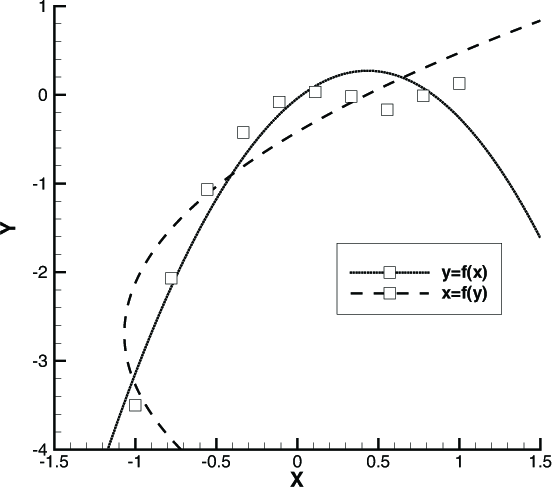
Figure 6-6. An XY Line plot type dependencies.
Similarly for Polar Line plots, the default setting is R=f(Theta) (you may change the value to Theta=f(R)). With R=f(Theta), the Theta-axis variable is the independent variable and the R-axis variable is the dependent variable. With Theta=f(R), the R-axis variable is the independent variable and the Theta-axis variable is the dependent variable.
To change the dependency setting:
1.From the Curves page of the Mapping Style dialog, select the mappings to change.
2.Right-click in the Dependent Variable column on the Curves page of the Mapping Style dialog choose either R=f(Theta) or Theta=f(R).
|
|
 For the XY Line plot type, the dependency setting determines the direction of bar charts. To create a vertical bar chart, set the dependency to
 Linear and polynomial fits allow you to specify a weighting variable. By default each data point is weighted equally. With the weighting variable, individual points can be given more or less weight. Relatively larger numbers in the curve weighting variable mean more significance for a given point. If the curve-weighting variable is zero at a data point, that data point has no effect upon the resulting curve. Therefore if your data contains outliers that would affect the overall curve fit, adding a zero weight at the point of the outlier will remove it from the overall curve fit calculation.
The weighting coefficients must be integers in the range of zero to 9,999. Weighting coefficients defined as floating-point numbers are truncated. That is, a weighting coefficient of 1.99 is truncated to 1.0.