20 - 1 Data Alteration through Equations
Use Data>Alter>Specify Equations (or click the  toolbar button) to alter data in existing zones. The dialog allows you to change the values of entire variables or specific data points. You can also use this dialog to create new variables.
Changes made to the dataset in the Specify Equations dialog are not made to the original data file. You can save the changes by saving a layout file or writing the new data to a file. Saving a layout file will keep your data file in its original state, but use journaled commands to reapply the equations.
|
|
 Variables defined in your data file, or variables you create yourself, are referenced in equations by surrounding them with curly braces, like {RPM}. This syntax must be used even when first defining a variable, for example {RPM} = {RPS} * 60 to define a new RPM variable from an existing RPS variable. Variable and function names provided by
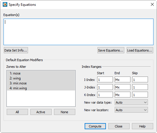
The Specify Equations dialog has the following options and fields:
• Equation(s) - Enter the equation(s) using the syntax described in Section 20 - 1.1 “Equation Syntax”.
• Data Set Info - Opens the Data Set Info dialog (see Section 5 - 4 “Data Set Information”).
• Save Equations - Save all equations in the Equation(s) field to a text file with an .eqn format.
• Load Equations - Load an equation file previously saved.
• Zones to Alter - Select which zones to alter. You can manually select the zones in the list (holding Shift when clicking to create a range, or Control to toggle individual zones on or off). You may use the buttons below the list to select all zones, all active zones, or no zones.
|
|
 When creating a new variable, if all zones are not selected, Tecplot will create a passive variable as a placeholder for any zones that are not included in the data alteration since all zones in a dataset must have the same number of variables. Passive variables effectively return zero for every point or cell value, do not consume any memory, and can be replaced at any time with other data alterations.
• Index Ranges - Select the index ranges to alter in the selected zones. You may skip this step if you want to apply the equation to all points of the selected zones. Use the special value 0 or Mx to specify the maximum index. You can also use the values Mx-1 (to specify the index one less than the maximum index), Mx-2, and so forth.
For Ordered Data, the I-Index, J-Index, and K-index options correspond to the I, J, and K values in the dataset. For finite element data, the I-Index corresponds to the range of nodes and the J-Index corresponds to the cell-centered values. The K-index has no bearing on finite element data.
The Skip field indicates the increment between indexes. 1 means apply the calculation to every data point, 2 means to every other data point, 3 to every third point, and so on. When creating a new variable, the new variable's value is set to zero at any index value that is skipped.
• New Var Data Type (if applicable) - Select the data type of the new variable. The following data types are available:
• Auto - Tecplot 360 EX assigns the data type based upon the variables used in the right-hand side of the equation.
• Single - Four-byte floating point values.
• Double - Eight-byte floating point values.
• Long Int - Four-byte integer values.
• Short Int - Two-byte integer values.
• Byte - One-byte unsigned integer values (can contain values from zero to 255).
• Bit - Either zero or one.
• New Var Location (if applicable) - Select the location of the new variable. The options are:
• Auto (default) - "Auto" is set to node unless all variables in the equation are located at the cell center.
• Node
• Cell-Center
• Compute - Click the Compute button to alter the data. If an error occurs during the alteration (because of division by zero, overflow, underflow, etc.), an error message is displayed, all of the zones are restored to their previous state as of the beginning of processing that equation, and processing stops. The results of equations that have been successfully processed, however, are retained.
For example, if you enter three equations, and the second contains an error, the final state is the result of processing only the first equation. The second equation is rolled back due to the error, and the third is not processed at all.
|
|
 Every time you hit the [Compute] button, the equations are calculated. Be sure to remove previously computed equations before computing new ones.
You can enter multiple equations in the Equation(s) text field of the Specify Equations dialog. Each equation occupies one line of the text field as demarcated by the Enter key (not necessarily by where they wrap in the text field). The equations are applied in order to all specified zones and data points.
Tecplot 360 EX equations have the following form:
LValue = F(RValue1, RValue2, RValue3,...)
Where: F() - A mathematical expression.
LValue - An existing or new variable.
RValueN - A value (such as a constant, variable value, or index value).
If LValue already exists in the dataset of the active frame, the equation is used to modify that variable. (The same variable may be used on the right side of the equation to refer to the pre-calculation value and thereby modify it based on its original value.) If the variable does not already exist, the equation is used to create a new variable as a function of existing variables.
There may be any number of spaces within the equation. However, there cannot be any spaces between the letters of intrinsic-function names nor in variables referred to by name. (See Equation Operators and Functions.)
A variable is specified in one of the following ways:
• Its order in the data file - A variable may be referenced according to its order in the data file, where V1 is the first variable in the data file, V2 is the second, and so forth.
To create a new variable using this specification, you must specify the number of the next available variable (i.e. if there are 5 variables in the dataset), the new variable must be called V6. You will receive an error message, if you attempt to assign an invalid variable number.
|
|
 You can confirm the number and order of variables in the data file in the
 • By its name - To reference a variable by its name, enclose the name with curly braces ("{" and "}"). For example, to set V3 equal to the value of the variable named R/RFR, you can enter:
V3 = {R/RFR}
Variable names are not case sensitive. Leading and trailing spaces are also not considered. However, spaces within the variable name are significant.
If two or more variables have the same name, the first variable is used when the variable is referred to by name. So, if both V5 and V9 are named R/rfr, V5 is used.
The curly braces can also be used on the left-hand side of the equation. In this case, if a variable with that name does not exist, a new variable is created with that name for all zones.
• By a letter code - Variables and index values may be referenced by the following letter codes:
• I - For I-ordered and finite-element data:
|
|
Finite-element |
Ordered |
|
Nodal |
J is equal to 1 |
I is equal to the I-index number |
|
Cell-centered |
J is equal to the element number |
I is equal to the I-index number |
• J - For J-ordered and finite-element:
|
|
Finite-element |
Ordered |
|
Nodal |
I is equal to the node number |
J is equal to the J-index number |
|
Cell-centered |
I is equal to 1 |
J is equal to the J-index number |
• K -
|
|
Finite-element |
Ordered |
|
Nodal |
K is equal to 1 |
K is equal to the K-index number |
|
Cell-centered |
K is equal to 1 |
K is equal to the K-index number |
For K-ordered and finite-element:
• X - The variable assigned to the X-axis. In XY-plots, all active mappings must have the same X-variable in order for this variable name to be valid.
• Y - The variable assigned to the Y-axis. In XY-plots, all active mappings must have the same Y-variable in order for this variable name to be valid.
• Z - The variable assigned to the Z-axis (if in 3D Cartesian).
• A - The variable assigned to the Theta-axis for Polar plots. For this variable to be valid, the plot type must be set to Polar Line. In addition, all active mappings must have the same Theta-variable.
• R - The variable assigned to the R-axis for Polar plots. The plot type must be Polar Line, and all active mappings must have the same R-variable for this variable name to be valid.
• U - The X-component of vectors (if defined).
• V - The Y-component of vectors (if defined).
• W - The Z-component of vectors (if defined).
• B - The value-blanking variable for the first active constraint (if applicable).
• C - The contour variable for contour group 1 (if defined in the Contour Details dialog).
• S - The scatter-sizing variable (if defined in the Scatter Size/Font dialog).
• SOLUTIONTIME - The current solution time.
• ZONENUM - The current zone number.
Letter codes may be used anywhere on the right-hand side of the equation. Do not enclose them in curly braces.
Those letter codes representing variables (all letter codes except I, J, and K) may be used on the left-hand side of the equation as well.
The variables referenced by the letter codes are for the current frame.
Equation Operators and Functions
Binary Operators
In an equation, the valid binary operators are as follows:
|
+ |
Addition |
|
- |
Subtraction |
|
* |
Multiplication |
|
/ |
Division |
|
** |
Exponentiation |
Binary operators have the following precedence:
|
** |
Highest precedence |
|
*,/ |
|
|
+,- |
Lowest precedence |
Operators are evaluated from left to right within a precedence level.
Functions
The following functions are available. Arguments may be variables, constants, expressions, other functions.
|
SIN(X) |
Sine of X (must be specified in radians) |
|
COS(X) |
Cosine of X (must be specified in radians) |
|
TAN(X) |
Tangent of X (must be specified in radians) |
|
ABS(X) |
Absolute value of X |
|
ASIN(X) |
Arcsine of X (result given in radians) |
|
ACOS(X) |
Arccosine of X (result given in radians) |
|
ATAN(X) |
Arctangent of X (result given in radians) |
|
ATAN2(A,B) |
Arctangent of A/B (result given in radians) |
|
SQRT(X) |
Returns the positive square root of X |
|
LOG(X), ALOG(X)a |
Natural logarithm (base e) of X |
|
LOG10(X), ALOG10(X)b |
Logarithm base 10 of X |
|
EXP(X) |
Exponentiation (base e); EXP(X)=e**X |
|
MIN(A, B) |
Minimum of A or B |
|
MAX(A, B) |
Maximum of A or B |
|
SIGN(X) |
Returns -1 if X is negative, +1 otherwise |
|
ROUND(X) |
Round X to the nearest integer |
|
TRUNC(X) |
Remove fractional part of X |
|
RAND(N) |
Returns random number between 1 and N inclusive, different for each element in the variable |
Conditional Expressions
Conditional expressions may be written using the IF function.
|
IF(P,T,F) |
If the predicate expression P is true (has a non-zero value), returns the value of expression T, otherwise returns the value of expression F. Both T and F are fully evaluated regardless of the value of P; there is no "short-circuiting." |
The predicate expression may include comparison and Boolean operators, as summarized in the following table.
|
Operator |
Description |
Example |
|
== |
Equal To |
{A} = IF(X==2.0, 3, 4) assigns to variable A: 3 if X equals 2.0, otherwise 4 |
|
!= |
Not Equal To |
{A} = IF(X != Y,Z,2) assigns to variable A: Z if X does not equal Y, otherwise 2 |
|
> |
Greater Than |
{A} = IF(X > 1.0, 4, 5) assigns to variable A: 4 if X > 1.0, otherwise 5 |
|
>= |
Greater Than or Equal To |
{A} = IF(X >= Y, 4, Z) assigns to variable A: 4 if X >= Y, otherwise Z |
|
< |
Less Than |
{A} = IF(X < Y, 4, Z) assigns to variable A: 4 if X < Y otherwise Z |
|
<= |
Less Than or Equal To |
{A} = IF(X <= Y, 4, Z) assigns to variable A: 4 if X <= Y, otherwise Z |
|
&& |
Logical AND |
{A} = IF(X < Y && X > 3, 8,9) assigns to variable A: 8 if X < Y AND X > 3, otherwise 9 |
|
|| |
Logical OR |
{A} = IF(X == 2 || X > 3, 5,6) assigns to variable A: 5 if X == 2 OR X > 3, otherwise 6 |
These operators are valid only within the first argument of an IF function. They may not be used elsewhere in an expression. For example, {A} = X > 1 is invalid. Instead, use {A} = IF(X > 1, 1, 0) or similar.
Python-style operator chaining (such as A < B < C) is not supported. Although this construction is syntactically valid, it will not produce the expected result. Use A < B && B < C instead.
&& has a higher precedence than (will be evaluated before) ||. When in doubt, use parentheses.
Derivative and Difference Functions
The derivative functions can be called in the same manner as intrinsic functions. Derivative and difference functions can be calculated with respect to the following variables:
|
Variable |
Definition |
Restricted to: |
|
x, y, z |
variable assigned to the x-axis, y-axis or z-axis, respectively |
XY Linea, or 3D |
|
a |
variable assigned to the theta-axis |
Polar Line |
|
r |
variable assigned to the radial-axis |
Polar Line |
|
i, j, k |
index range |
Ordered Zones |
|
aIf you have multiple x-axes or y-axes in an XY line plot, the variables assigned to the x and y-axis in the first available mapping will be used. |
The complete set of first and second-derivative and difference functions are listed below:
|
Type |
Function Calls |
Applicable Variables |
|
First Order |
ddx, ddy, ddz, dda, ddr |
x, y, z, a, or r |
|
Second Order |
d2dx2, d2dy2, d2dz2, d2da2, d2dr2 |
x, y, z, a or r |
|
Second-Order (cross derivatives) |
d2dxy, d2dyz, d2dxz, d2dar |
xy, yz, xz, or ar |
The derivative function ddx is used to calculate ; d2dx2 calculates
  ;
;
and d2dxy calculates  .
.
|
Type |
Function Calls |
Applicable Variables |
|
First Order |
ddi, ddj, ddk |
i, j, or k |
|
Second Order |
d2di2 d2dj2, d2dk2 |
i, j, or k |
|
Second Order (cross derivatives) |
d2dij, d2djk, d2dik |
ij, jk, or ik |
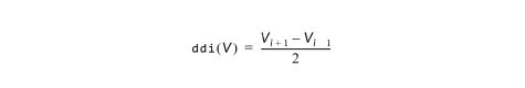
The difference functions ddi, d2di2, and so forth, calculate centered differences of their argument with respect to the indices I, J, and K based on the indices of the point. For example:
For ordered zones, spatial derivative functions are calculated using the chain rule with difference functions. For example:

or:

The spatial derivatives of indices, such as ddx(i), are calculated from their inverses, such as ddi(x), using standard curvilinear coordinate transformations.
For finite-element zones, spatial derivatives are calculated using the Moving Least-Squares technique. The variable at a particular node or cell center is assumed to vary quadratically in space about that point, and least-squares is used with all nodes surrounding the point to fit a polynomial function, whose coefficients then become the first and second derivatives of the variable.
Boundary values for first-derivative and difference functions (ddx, ddy, ddz, ddi, ddj, and ddk) of ordered zones are evaluated in one of two methods: simple (default) or complex1.
For simple boundary conditions, the boundary derivative is determined by the one-sided first derivative at the boundary. This is the same as assuming that the first derivative is constant across the boundary (i.e., the second derivative is equal to zero).
For complex boundary conditions, the boundary derivative is extrapolated linearly from the derivatives at neighboring interior points. This is the same as assuming that the second derivative is constant across the boundary (i.e. the first derivative varies linearly across the boundary).
For second-derivatives and differences (d2dx2, d2dy2, d2dz2, d2dxy, d2dyz, d2dxz, d2di2, d2dj2, d2dij, d2dk2, d2djk, and d2dik), these boundary conditions are ignored. The boundary derivative is set equal to the derivative that is one index in from the boundary. This is the same as assuming that the second derivative is constant across the boundary.
|
|
 You can create your own derivative boundary conditions by using the index range and the indices options discussed previously.
The use of derivative and difference functions is restricted as follows:
• Derivatives and differences for IJK-ordered zones are calculated for the full 3D volume. The IJK-mode for such zones is not considered.
• If the derivative cannot be defined at every data point in all the selected zones, the operation is not performed for any data point.
• Derivative functions are calculated using the active frame's axis assignments. Be careful if you have multiple frames with different variable assignments for the same dataset.
• Derivatives at the boundary of two zones may differ since Tecplot 360 EX operates on only one zone at a time while generating derivatives.
Use the Analyze menu to calculate integrals with Tecplot 360 EX. See Section 21 - 7 “Performing Integrations” for information.
You may use auxiliary data containing numerical constants in equations. The syntax for using auxiliary data in equations is:
AUXZONE[nnz]:Name
AUXDATASET:Name
AUXFRAME:Name
AUXVAR[nnv]:Name
AUXLINEMAP[nnm]:Name
where
nnz = the zone number(s)
nnv = the variable number(s)
nnm = the line map number(s)
Name = name of the auxiliary data
For example, a dataset auxiliary data constant called Pref would be referenced using AUXDataSet:Pref. Equations using this auxiliary data might appear as:
{P} = {P_NonDim} * AUXDataSet:Pref
20 - 1.4 Zone Number Specification
By following a variable reference with square brackets ("[" and "]"), you can specify a specific zone from which to get the variable value.
The zone number must be a positive integer constant less than or equal to the number of zones. The zone specified must have the same structure (I, IJ, or IJK-ordered or finite element) and dimensions (IMax, number of nodes) as the zone(s) the equation(s) will be applied to.
|
|
 If you do not specify a zone, the zone modified by the left-hand side of the equation is used.
Zone specification works only on the right-hand side of the equation.
By following a variable reference with parentheses, you can specify indices for ordered data only. Indices can be absolute or an offset from the current index.
Index offsets are specified by using the appropriate index "i", "j" or "k" followed by a "+" or "-" and then an integer constant. Any integer offsets may be used. If the offset moves beyond the end of the zone, the boundary value is used. For example, V3(i+2) uses the value V3(IMAX) when I=IMax-1 and I=IMax. V3(I-2) uses the value of V3(1) when I=1 or I=2.
Absolute indices are specified by using a positive integer constant only. For example, V3(2) references V3 at index 2, regardless of the current i index.
If the indices are not specified, the current index values are used.
20 - 1.6 Variable Sharing Between Zones
For zones with the same structure and index ranges, you can set a variable to be shared by specifying that the variable for those zones have the values from one zone. For example, if zones 3 and 4 have the same structure and you compute V3=V3[3] for zones 3 and 4, V3 will be shared.
|
|
 Subsequent alteration of the variables may result in loss of sharing.
The zone and index restrictions specified in the Specify Equations dialog can be overridden on an equation by equation basis. To specify restrictions for a single equation add the colon character (:) at the end of the equation followed by one or more of the following:
|
Equation Restrictor |
Comments |
|---|---|
|
<Z=<set>> |
Restrict the zones. |
|
<I=start[,end[,skip]]> |
Restrict the I-range. |
|
<J=start[,end[,skip]]> |
Restrict the J-range. |
|
<K=start[,end[,skip]]> |
Restrict the K-range. |
|
<D=datatype> |
Set the data type for the variable on the left hand side. This only applies if a new variable is being created. |
|
<V=valuelocation> |
Set the value location (NODAL or CELLCENTERED) for the variable on the left hand side. Only applicable if a new variable is being created. |
For example, to add one to X in zones 1, 3, 4, and 5:
X=X+1:<Z=[1,3-5]>
The following example adds one to X for every other I-index. Note that zero represents the maximum index.
X=X+1:<I=1,0,2>
The next example creates a new variable of type Byte:
{NewV}=X-Y:<D=Byte>
Tecplot 360 EX allows you to put your equations in macros. A macro with just equations in it may be referred to as an equation file, and in fact equation files saved using the Save Equations button are macro files with an .eqn extension. An equation in a macro file is specified using the $!ALTERDATA macro command. Equation files may also include comment lines and must start with the comment #!MC 1410, like other macro files. If you are performing complex operations on your data, and/or the operations are repeated frequently, equation files can be very helpful.
You can create equation files from scratch using an ASCII text editor, or you can create your equations interactively by using the Specify Equations dialog and then save the resulting equations. The standard file name extension for equation files is .eqn.
For example, you might define an equation to compute the magnitude of a 3D vector. In the Specify Equations dialog, it would have the following form:
{Mag} = sqrt(U*U + V*V + W*W)
In a macro file, it would have the following form:
#!MC 1410
$!ALTERDATA
EQUATION = "{Mag} = sqrt(U*U + V*V + W*W)"
The interactive form of the equation must be enclosed in double quotes and supplied as a value to the EQUATION parameter of the $!ALTERDATA macro command.
To read an equation file, select Load Equations on the Specify Equations dialog. In the Load Equation File dialog, select an equation file that contains a set of equations to apply to the selected zones of your data. The equations in the equation file will be added to the list of equations in the dialog. All equations are applied to your data when you click Compute.
Equations in equation files may be calculated somewhat differently depending on whether the computation is done from within the Specify Equations dialog or by running the equation file as a macro. When loaded into the Specify Equations dialog, equations that do not contain zone or index restrictions use the current zone and index restrictions shown in the dialog. When processed as a macro file, the equations apply to all zones and data points. To include zone and index restrictions, you must include them in the equation file as part of the $!ALTERDATA command.
Refer to the Scripting Guide for more information on working with the $!ALTERDATA command.
In the following equation, V1 (the first variable defined in the data file) is replaced by two and a half times the existing value of V1:
V1 = 2.5*V1
The following equation sets the value of a variable called Density to 205. A new variable is created if a variable called Density does not exist.
{Density} = 205
In the next equation, the values for Y (the variable assigned to the Y-axis) are replaced by the negative of the square of the values of X (the variable assigned to the X-axis):
Y = -X**2
The following equation replaces the values of V3 with the values of V2 rounded off to the nearest integer. A new variable is created if there are only two variables currently in the data set.
V3 = round(V2)
In the following equation, the values of the fourth variable in the data set are replaced by the log (base 10) of the values of the third variable.
V4 = ALOG10(V3)
Suppose that the third and fourth variables are the X and Y-components of velocity and that there are currently a total of five variables. The following examples create a new variable (V6) that is the magnitude of the components of velocity.
V6 = (V3*V3+V4*V4)**0.5
or
V6 = sqrt(V3**2+V4**2)
You can also accomplish the above operation with the following equation (assuming you have already defined the vector components for the active frame):
{Mag} = sqrt(U*U + V*V)
The following equation sets the value of a variable named diff to the truncated value of a variable named depth subtracted from the existing value of depth:
{diff} = {depth} - trunc({depth})
In the next equation, C (the contour variable) is set to the absolute value of S (the scatter-sizing variable), assuming both C and S are defined:
C = abs(S)
In the following example, a new variable is created (assuming that only seven variables initially existed in the data file). The value for V8 (the new variable) is calculated from a function of the existing variables:
V8 = SQRT((V1*V1+V2*V2+V3*V3)/(287.0*V4*V6))
The above operation could have been performed in two simpler steps as follows:
V8 = V1*V1+V2*V2+V3*V3
V8 = SQRT(V8/(287.0*V4*V6))
The following equation replaces any value of a variable called TIME that is below 5.0 with 5.0. In other words, the values of TIME are replaced with the maximum of the current value of TIME and 5.0:
{TIME} = max({TIME},5)
The following equation creates variable V4 which has values of X at points where X<0; at other points, it has a value of zero (this does not affect any values of X):
V4 = min(X,0)
Another example using intrinsic functions is shown below:
V8 = 55.0*SIN(V3*3.14/180.0) + ALOG(V4**3/(v1+1.0))
You can also reference the I, J, and K-indices in an equation. For example, if you wanted to cut out a section of a zone using value blanking, you could create a new variable that is a function of the I and J-indices (for IJ-ordered data). Then, by using value-blanking, you could remove certain cells where the value of the value-blanking variable was less than or equal to the value blanking cut-off value.
Here is an example for calculating a value-blanking variable that is zero in a block of cells from I=10 to 30, and is equal to one in the other cells:
V3 = min((max(I,30)-min(I,10)-20),1)
The following equation replaces all values of Y with the difference between the current value of Y and the value of Y in zone 1. (If zone 1 is used for the data alteration, the new values of Y will be zero throughout that zone.)
Y = Y - Y[1]
The following equation replaces the values of V3 (in an IJ-ordered zone) with the average of the values of V3 at the four adjacent data points:
V3 = (V3(i+1,j)+V3(i-1,j)+V3(i,j+1)+V3(i,j-1))/4
The following equation sets the values of a variable called TEMP to the product of the values of a variable called T measured in four places: in zone 1 at two index values before the current data point, in the current zone at an absolute index of three, in zone 4 at the current data point, and in the current zone at the current data point.
{TEMP} = {T}[1](i-2) * {T}(3) * {T}[4] * {T}
Indices may be combined with zone specifications. The zone is listed first, then the index offset. For example:
V3 = V3 - V3[1](i+1)
Y = Y[1] - Y[2](1) + Y(1,j+3) + Y
Referencing variables by letter code:
V3 = I + J
V4 = cos(X) * cos(Y) * cos(Z)
{Dist} = sqrt(U*U + V*V + W*W)
{temp} = min(B,1)
Specifying the Zone number for a given variable:
V3 = V3 - V3[1]
X = ( X[1] + X[2] + X[3] ) / 3
{TempAdj} = {Temp}[7] - {Adj}
V8 = V1[19] - 2*C[21] + {R/T}[18]